
Quantum Algorithm for Combinatorial Optimization
The combinatorial optimization is one of the most promising fields of quantum algorithms. Among the various predictions about futures of the quantum computers, people have said that at least the quantum computers can solve the combinatorial problems much faster than the classical computers.
In this posting, we’ll see the algorithm to solve the combinatorial problems from classical algorithms including simulated annealing and genetic algorithm to quantum algorithms including quantum annealing and quantum approximated optimization algorithm (QAOA)
$\def\ket#1{\mid #1 \rangle}$
1. Combinatorial Problem
The usual mathematical problems have continuous solution set and therefore their objective functions have continuous surface. This means that we can calculate the gradients which give useful hints about the optimal points. In this case, we usually assume that our objective function is convex or locally convex and use gradient based methods including gradient descent or newton’s methods. The detailed explanations about convex optimization is in here.
On the other hand, the feasible solution sets of the combinatorial problems are discrete. Therefore, the surface of the objective function moves discontinuously and cannot get the gradients. So we cannot use the useful and powerful techniques of the convex optimization.
For example, there is a max-cut problems. Assume we have graph which consists of 5 vertices (or nodes) and several edges (or links). We can paint the vertices with red or blue and want to know that which combinations could make largest numbers of line between different color.
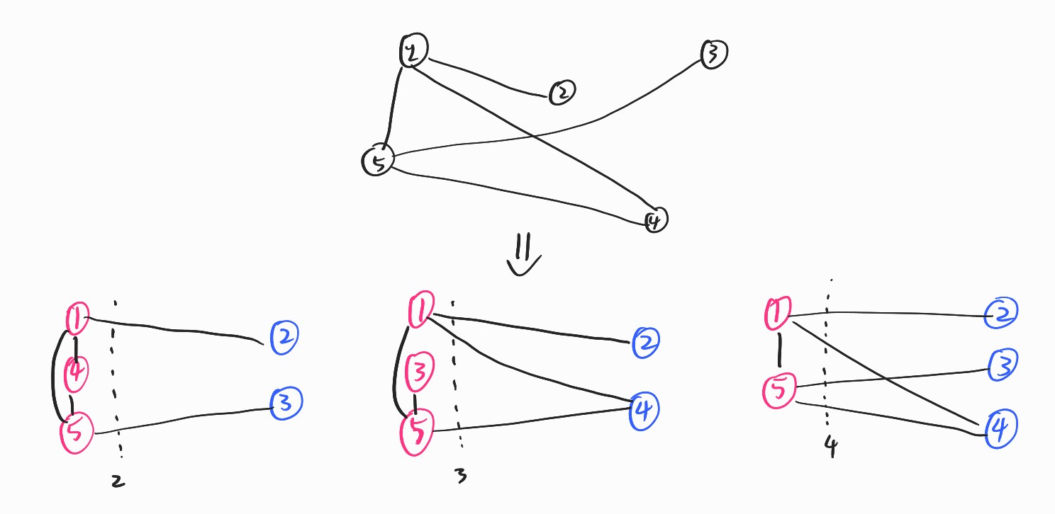
As we see that, to get the exact optima of the problems, we have to test $2^5$ numbers of the combinations. If we have $n$ numbers of vertices, than we have to test $2^n$ numbers of the cases so it is NP problem.
We can formulate the problems as follows \(\max f(x_1,x_2,...,x_n) \\ \mbox{where } x_{i} \in \{0,1,...,n_i\}\) Remark that we cannot get $\nabla f(x)$ because it is not continuous in a sense of $\mathbb{R}^n$.
2. Classical Algorithms to solve the combinatorial optimization
There are several classical algorithm to solve the combinatorial optimizations. We’ll see two basic algorithms called genetic algorithm and simulated annealing. Both of them assume that two combination with similar pattern have similar objective values or, at least they are not that different.
This could be interpreted as weak continuity. Remark that the definition of the continuous is for all epsilon, there is a delta such that $d(x,y) <\delta$ implies $d(f(x),f(y)) <\epsilon$. The pattens and the values could be interpreted as input and output of the functions. We may interpret the assumption as a modified version of the continuous which replace the all $\epsilon$ conditions into for all $\epsilon>c$ for some constant $c$. It means weak bonds
A. Genetic Algorithm
Genetic Algorithm are intuitive algorithms which mimic the genetic evolution procedures. It has three procedures containing Selection, Crossover and Mutation.
Let assume we have to find 20 numbers of parameters $(x_1,x_2,…x_{20}), x_i\in {0,1}$. To get the global optima, we have to evaluate $2^{20} \approx 1,000,000$ numbers of cases which takes too many times.
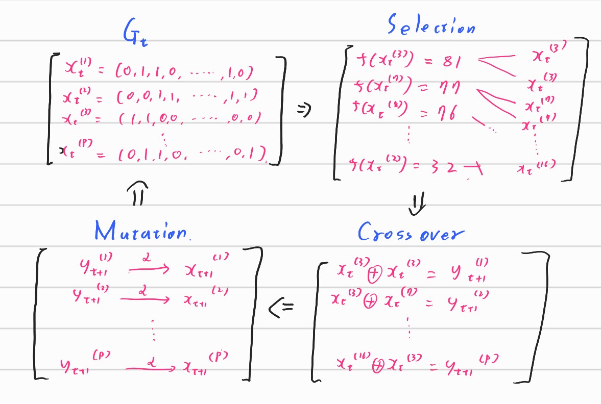
We will make t-th Generation $G_t$ which consist of $P$ numbers of combinations. The number $P$ is called as size of Population. We’ll evolve the generation using the three procedure and make the generation better and better to get the best objective values.
0. Initialization
- First of all, it randomly makes $P$ numbers of combinations using the parameters.
1. Selection
- In the selection procedure, it first evaluates each combination and it makes parent candidate pool with the criterion of the values.
- The detailed procedure is varied from the algorithms. We can select them with either weighted probabilities or fixed proportion.
2. Crossover
- In the crossover phase, we’ll mix the candidates of the parent pool into one.
- The detailed procedure could be varied from the algorithms. The most famous methods is using 80% of combinations of first parent and using 20% of combinations of second parent.
3. Mutation
- In the mutation procedure, each parameter flips with the predetermined probability of $\alpha$
- It is known that the mutation procedure makes the algorithm faster and more efficient.
And the result becomes next generation $G_{t+1}$ and keep going until it finds good combinations.
Intuitively, we could expect that the algorithm could give us quite a good candidates of combinations. Each procedure could be interpreted with mathematical intuition. Let’s see them after we see the simulated annealing.
B. Simulated Annealing
Annealing is a technique to handle the iron. By repeating heating up and ising down the iron, we can get intended shape and much more strong iron. Similar with the real annealing, the simulated annealing has heating up and ising down procedures.
The most basic procedure has two stages.
0. Initialization
- First of all, it takes random starting point of $x_0$
1. Proposal Stage
- Propose new candidates $x_{t+1}’$ using proposal function $k(x_{t}, x’_{t+1})$.
- The proposal function could be varied from the algorithms but the Markov Chain Monte Carlo (MCMC) using probability distribution function such as gaussian distribution or exponential distribution to propose random candidates.
2. Acceptance Stage
- Evaluate the ratio between $f(x_{t})$ and $f(x_{t+1}’)$. If the evaluation values of new candidate is relatively large enough, then it accept the values and regard $x_{t+1}$. If the values are not that high, then it reject the candidates and takes new values.
- The detailed procedure of the usual MCMC in Bayesian methods is regard the ratio $\frac{f(x_{t+1}’)}{f(x_t)}$ as probability and compare it with randomly chosen numbers in $(0,1)$. Therefore, the MCMC accept the candidates probabilistically.
We can regard the proposal stage as heating up and acceptance stage as ising down. Let’s see below figure. We can regard the objective function of combinatorial optimization problem as a function with too many local optima.
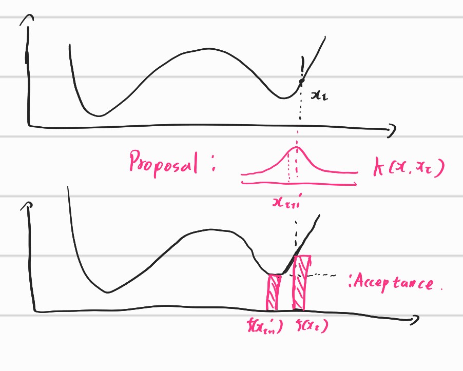
Usually, we regard the function as temperature or energy. In the figure, we have to accept reasonable candidates to go down the hill which could be interpreted as ising procedure. However, the global optima lies in beyond the hill. Therefore, we have to consider the candidates beyond the hill. This procedure could be done with proposal procedure. By propose new candidates over the hill, it can suggest new potential patterns of true solutions.
By combining both methods, we can interpret them intuitively.
- First of all, the combinatorial optimization problems could be regarded as problems with too many local optima
- To find minimal values, we have to explore new candidates gradually not that far from current candidates. This is because of the weak continuity. Among huge candidates, the most reasonable candidates is a candidates similar with current best parameters.
- In the genetic algorithm, it is implemented as selection stage and crossover. It uses candidates having good evaluation values and mixes them.
- In the simulated annealing, the usual proposal functions propose the values near the current values and the acceptance procedure accepts the candidates by evaluating function.
- However, to overcome the local optima, we have to consider the candidates far form the reasonable candidates. This means that even though our result is $(2,3)$ in a sense of convexity, we have to consider new candidates far form the results such as $(10,0), (-7,8)$ or $(6,-5)$.
- In the genetic algorithm, it is done using crossover and mutation. By crossover, it explore whole new candidates. By mutation, it also explore new potential candidates.
- In the simulated annealing, even though the probability might not that high, the proposal function could propose new candidates far from the current values. Also, the acceptance procedure could accept new values even though the values are not that good compared with the current values.
Therefore, we can interpret that the optimizing the combinatorial problems usually consists with two dogma that exploring reasonable candidates using the continuity of the problems and exploring unreasonable candidates considering the discontinuity of the problems.
3. Quantum Algorithms to solve the combinatorial optimization
A. Quadratic Unconstrained Binary Optimization (QUBO)
Now, let's see the quantum algorithms to solve the combinatorial algorithms. Basically, all of them are based on the quantum annealing.
There is a base problem of most of the quantum annealing problem.
Quadratic Unconstrained Binary Optimization (QUBO)
$\max x^t Q x + \beta^t x \mbox{ subject to } x \in {0,1}^n$
We can easily expand the QUBO in to more specific problem. For example, we can expand the binary conditions into integer or continuous with one hot encoding. Or, we can transform the traveling salesman's problem (TSP) into QUBO form. We'll see the detailed example at next post.
In the quantum Algorithms, we have to embed the problems into Hamiltonian form. For the mathematician, Hamiltonian could be understood as operator of quantum. Because quantum theory is based on the Euclidean Hilbert Space, the Quantum is vector and the Hamiltonian is matrix.
Let write the $x$ into binary digit $x= x_0x_1x_2 … x_{n-1}$ where $x_i \in {0,1}$. In quantum computer, we can write $\ket{x} = \ket{x_0x_1…x_{n-1}} = \ket{x_0}\ket{x_1}…\ket{x_{n-1}}$.
Then we will use following equations and definitions
- $c(x) = x^{\dagger}Qx + \beta^{\dagger}x = \sum_{i,j}q_{ij}x_ix_j + \sum_{i} \beta_i x_i$
- $Z_i := I^{\otimes i-1}Z I^{\otimes n-i}$
- $Z_i \ket{x} = (-1)^{x_i}\ket{x} = (1-2x_i)\ket{x}$
The $Z_i$ in the definition (2) is simple operator apply $Z$ gate only at i-th qubit. Remark that $Z_iZ_j = I^{\otimes i-1}ZI^{\otimes j-i-1} Z I^{\otimes n-j}$ which means applying $Z$ gate at i-th and j-th qubits.
Because $Z \ket{0} =\ket{0}$ and $Z\ket{1} = -\ket{1}$, we can write $Z_i \ket{x} = (-1)^{x_i}\ket{x}$.
Using the equation (3), we can write $x_i \ket{x} = \frac{I-Z_i}{2}\ket{x}$ and $x_ix_j \ket{x} = \frac{I-Z_i}{2}\frac{I-Z_j}{2}\ket{x}$ \(\begin{align*} c(x)\ket{x} &= \sum_{i,j}q_{i,j}x_ix_j\ket{x} + \sum_{i}\beta_i x_i\ket{x} \\ &=\sum_{i,j}q_{ij} \frac{I-Z_i}{2}\frac{I-Z_j}{2}\ket{x} + \sum_{i}\beta_i \frac{I-Z_i}{2}\ket{x} \\ &= \left[ \frac{1}{4} \sum_{i}\sum_{j} q_{ij}Z_i Z_j -\frac{1}{2} \sum_{i}(\beta_i + \sum_{j}q_{ij})Z_i +\frac{1}{4} \sum_i(\sum_j q_{ij}+2\beta_i)I\right] \ket{x} \\ & =: H_P \ket{x} \end{align*}\)
Finally we can get the matrix returning the cost of the input vector i.e. $H_P\ket{x}=c(x) \ket{x}$. If we use the uniform superposition qubit $\ket{+}^{\otimes n} = \frac{1}{2^n}\sum_{j=0}^{2^n-1}\ket{j}$, then we can get $H_P\ket{+}^{\otimes n} = \sum_{j=0}^{2^n-1} \frac{c(j)}{2^n}\ket{j}$. This means that the most frequently returned outcome is the optimal parameter because the probabilities of each outcome are $\frac{c^2(j)}{2^{n+1}}$. However, with several technical and theoretical problems, we cannot directly use the results. We have to use another techniques called as quantum annealing.
B. Quantum Annealing
Remark that annealing algorithm is based on the energy function. Therefore, in actually, it concerns the energy of some quantum states. It is based on the Shrodinger's Formula \(i \frac{d \ket{\psi(t)}}{dt} = H(t) \ket{\psi(t)}\) Which states that the movement of some quantum could be determined using matrix valued function $H(t)\ket{\psi(0)} = \ket{\psi(t)}$. Let define $H(t) \ket{\psi_j(t)} = \epsilon_j(t) \ket{\psi_{j}(t)}$ which is $\epsilon_j(t)$ is eigenvalue and $\ket{\psi_{j}(t)}$ is eigenstate of the Hamiltonian.
There is a famous theorem which is essential to quantum annealing.
Adiabatic Theorem
$\ket{\psi_{j}(0)}$ remain in $\ket{\psi_j ( s)}$ for all $s \in [0,1]$ where $s = t/T$ if $T » O(\mid \epsilon_j - \epsilon_k \mid ^{-2}),k\neq j$
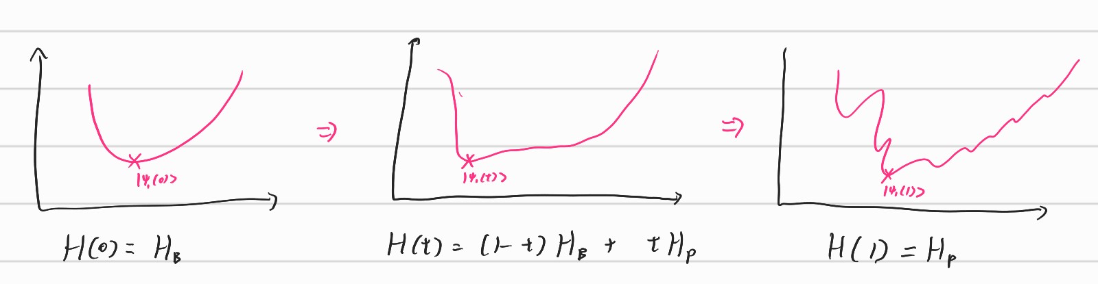
This means that if start with j-th eigenstate and really slowly evolve the state with $H(t)$, then the state always remain in the j-th eigenstate at whole time $t$.
Therefore, if we design $H(t) = (1-\frac{t}{T})H_B+\frac{t}{T}H_p$ where $H_B$ is easy Hamiltonian which we know the exact eigenstate and $H_P$ is problem Hamiltonian which is target problems.
Therefore, by using the procedure, we can find ground state (i.e. minimal eigenvalue of matrix) of problem Hamiltonian. This is called as quantum annealing.
We can interpret them as starting at the low resolution and gradually enlarging the resolution to achieve our true problems.
The D-WAVE quantum device is actually a computer to only handle this QUBO problems. Therefore, it could be seen as quantum annealer rather quantum computer. But even with the quantum annealer, we can do quite a lot of things.
One of the most big obstacle of quantum annealer is we don’t know the values of $T$. The $T$ corresponds to the gap between eigenvalues. In the sense of matrix, it is a gap between largest eigenvalues and smallest eigenvalues i.e. the size of the spectrum of the matrix. To achieve the eigenstate, we have to use long $T$ and more slowly evolves the system.
However, because we don’t know the quantity of the gap, we also cannot know ideal time $T$. So the problem is where to stop the evolution. This is named as Annealing Schedule.
C. Quantum Approximated Optimization Algorithm (QAOA)
The quantum approximated optimization algorithm is also algorithm to solve the combinatorial problems. Not like the quantum annealing, the QAOA algorithm is designed for quantum computers. This “quantum computer” means a circuit based universal quantum computer designed to handle much general problems.
The operator in the circuit based quantum computer have to be unitary. Therefore, we have to change the Hamiltonian into matrix exponential form. \(U_P = \exp (i \theta H_p) , U_B = \exp (i \theta H_B)\) The state after $T$ time with dependent Hamiltonian $H(t)$ have to be calculated as follow. \(U(T,0) = \mathcal{J} \exp \left[-i \int_0^T H(t) dt\right]\) It is obvious from the Shrodinger’s equation. \(i \frac{\delta \psi}{\delta t} = H(t)\psi(t) \\ \int_{\psi(0)}^{\psi(T)} d \psi = -i \int_0^T H(t) \psi(t) dt \\ \psi(T) - \psi(0) = -i \int_0^T H(t)\psi(t) dt \\ \Rightarrow H(T,0) := -i \int_0^T H(t) dt \\ U(T,0) = \mathcal{J} \exp \left[-i \int_0 ^T H(t) dt\right]\) Therefore, to get the result of the evolution, we have to calculate the integral which is too complicated one.
In this cases, we can assume that our Hamiltonian is piecewise constant. Then, we can handle the hamiltonian as follow. \(U(T,0) = \exp \left[ i \sum_{j=1}^N \Delta t H(j \Delta t)\right]\) This is a simple numerical integration.
To implement it in the circuit based computer, we need little bit technical approaches.
In the usual quantum computer, we can implement arbitrary $2 \times 2$ unitary matrix $U$ with Pauli operators \(U = \alpha \sigma_i + \beta \sigma_x + \gamma \sigma_y + \delta \sigma_z\) Similarly, we can implement any arbitrary $2^n \times 2^n$ unitary matrix using the basis set ${\sigma_i,\sigma_x,\sigma_y,\sigma_z}^{\otimes 2^n}$ and $CNOT$ gate.
Let’s only think about $2 \times 2$ cases. Assume we want to implement $e^{iUt}$ and know the coefficient $\alpha,\beta ,\gamma$ and $\delta$.
Then we can decompose the U as follow \(e^{iUt} = e^{i\alpha\sigma_i + i\beta\sigma_x + i \gamma \sigma_y + i \delta \sigma_z } \\ = e^{i \alpha \sigma_i}e^{i\beta \sigma_x}e^{i\gamma \sigma_y} e^{i \delta \sigma_z} \\ = R_x(\beta) R_y(\gamma )R_z(\delta)\) The $R_x (\theta)$ is rotation gate which is implemented physically in the quantum devices. In the quantum device, there are only a few gates $I,Z,CNOT,R_X$. Other gates are implemented using the combination of the above gates.
The detailed components such as bases or physical gates might be different because there are more better approximation approaches. However, the core ideas is same.
However, the above equations do not hold in actually. Because each of the matrix does not have commutativity i.e. $AB \neq BA$, the equation $e^{A+B} =e^Ae^B$ usually do not hold.
Therefore, we need additional theorem.
Trotter-Suzuki Formula
$\exp \left[ -i \sum_{k=1}^m H_kt\right] = \prod_{k=1}^m \exp \left[-i H_kt\right] +O(m^2t^2)$
It means that we can use the approximated equation $e^{A+B}=e^Ae^B$ if we slowly apply the matrix operator. For the most easiest form, below equation holds. \(e^{A+B} = \lim_{n\rightarrow \infty} \left(e^{\frac{A}{n}} e^{\frac{B}{n}}\right)^n = e^{\frac{A}{n}}e^{\frac{B}{n}}e^{\frac{A}{n}}e^{\frac{B}{n}}....e^{\frac{A}{n}}e^{\frac{B}{n}}\)
Finally, we can get the QAOA algorithm as follow. \(U(T,0)\ket{+}^{\otimes n} \approx \prod_{j=1}^N\left[ \exp \left[-i \beta_j H_B\right]\exp \left[-i \gamma_j H_p \right]\right]\ket{+}^{\otimes n} := \ket{\beta,\gamma}\) The values of $\beta_j$ and $\gamma_j$ is target of optimization. We have to optimize them and get the optimal parameters.
That is, \(\underset{\beta,\gamma}{\min} \bra{\beta, \gamma} H_P \ket{\beta ,\gamma}\)
Until now, we have seen the quantum algorithm for combinatorial optimization. Because the algorithm could be applied at many fields, we can make a lot of academic researches using the algorithms.