
Chapter 3. Complex Number and Quantum Fourier Transformation
To implement the quantum algorithm, it is essential to understand the concept of the complex number. However, because the field of data science merely uses the complex number, most data scientists are not familiar with the complex number.
Therefore, to explore the quantum computer deeper, let’s study the complex number first.
1. The basic of the complex number
Definition of the complex number
The complex number is an extension of the real number and it is defined as follows.
$C := {z \mid z= a+bi,a,b\in R,i^2=-1}$
The character “i” in this definition is called an imaginary number and defined as the square root of the negative one.
For this definition, a is called a real part and denoted as Re(z) and b is called an imaginary part and denoted as Im(z). Therefore, every real number is a complex number with zero imaginary part.
In the real number space, the two elements in it can be ordered like $1<3$ or $-7.12 < \sqrt{5.66}$. However, in the complex number space, the order between imaginary numbers cannot be determined like between $i$ and $-i$ or between $3i$ and $12i$.
Therefore, the real space is an order field but the complex space is not an ordered field.
Moreover, the equation $z_1 = z_2$ is held if and only if equations $Im(z_1)=Im(z_2)$ and $Re(z_1)=Re(z_2)$ are held. It gives the intuition that the real part and the imaginary part can be taught as separate regions.
The basic operation of the complex numbers
- $0 = 0+0i$
- $1 = 1+0i$
- $-(a+bi)=-a-bi$
- $(a+bi)+(c+di)=(a+c)+(b+d)i$
- $(a+bi) \times (c+di) = (ac-bd)+(ad+bc)i$
- $Re((a+bi)\times(c+di))=ac-bd$
- $Im((a+bi)\times(c+di))=ad+bc$
The conjugate complex number
Conjugate means the other part of a pair. Therefore, the conjugate complex number can be understood as the other part which consists of a pair with an original complex number.
For a complex number $z = a+bi$, the conjugate of $z$ is denoted as $\bar{z}$ and calculated as $a-bi$
The reason why such a number is important is because the definition of the complex number is the square root of the negative one, and both $i$ and $-i$ fit the definition.
The conjugate complex number has following properties
- $z \bar{z} = a^2+b^2$ ; The product of complex number and its conjugate is non-negative real number
- $z=0$ iff $\bar{z} =0$
- $Re(z)=Re(\bar z) = a$
- $Im(z)=-Im(z)=b$
- If $Im(z)=0$, then $z=\bar{z}$
By using the conjugate complex number, we can calculate the inverse of a complex number like below.
$z^{-1}=\frac{1}{z}=\frac{\bar z}{\bar z z} = \frac{a-bi}{a^2+b^2} \\ \quad =\frac{a}{a^2+b^2} - \frac{b}{a^2+b^2}i$
The basic operation of the conjugate complex number is calculated as follows.
- $z = \bar{\bar{z}}$
- $\overline{z^{-1}}=\frac{1}{\bar{z}}$
- $\overline{z+w} = \overline{z}+\overline{w}$
- $\overline{z-w}=\overline{z}-\overline{w}$
- $\overline{z\times w} = \overline{z} \times \overline{w}$
Measurement of the complex number
The absolute value of the complex number can be defined by using the conjugate complex number as follow
$\mid z \mid = \sqrt{z\overline{z}}$
Therefore, we can apply p-norm in the real space using the definition,
$\parallel z \parallel_p = (\sum_{i=1}^n \mid z_i\mid^p)^{1/p} $
The complex Inner Product is defined as follows (Hermitian inner product).
$\left< z_1,z_2\right>=\sum_{i=1}^n z_{1i}\times \overline{z_{2i}}$
With the notation of matrix and vector, the inner product can be represented as follows.
$\left< z_1, z_2\right> = z_2^hz_1$
Superscript h means conjugate transpose which takes transpose and turn each element the conjugate complex number
Therefore, the L2-norm is defined as follows.
$\sqrt{z_2^hz_1}$
Moreover, by using the relation between Norm and Metric, it can be expanded to Metric
$(\parallel z_1-z_2\parallel_p)^{1/p}$
We can define the inner product as a hermitian inner product and can construct the Hilbert space naturally.
Like Euclidean space $\mathbb{R}^n $(;multiple real world), by using the Cartesian product, we can expand a single complex space $\mathbb{C}$ to a multiple complex space $\mathbb{C}^n$
2. Understanding the complex number
Complex plane and Polar Form
If we use the definition of the complex number $z=x+yi,(x,y \in \mathbb{R})$ and the separative property between real part and imaginary part, we can represent the complex number at 2-dimensional coordinate plane.

The figure is the result of replacing basis (1,0) and (0,1) which are the basis of the formal coordinate plane to (1,0) and (0,i). By using this, we can represent every element in $\mathbb{C}$.
But in this plane, we can use polar expression by using an angle and magnitude as $(r \cos \theta , r \sin \theta)$ and therefore,$z= x+yi = r\cos \theta +ri \sin \theta$.
If we tie up $r$ and apply the Euler’s formula to $\cos \theta + i \sin \theta$, then we can get the following expression.
$z= x+yi = r e^{i\theta}$
The former form $z = x+ yi$ is called the Cartesian Form and the latter form $z=r e^{i \theta}$ is called the Polar Form.
In the above figure, we can see that the conjugate of $z$ is rotating with $\theta$ in the counterclockwise direction and therefore, we can express it as follows.
$\overline{z} = x-yi = re^{-i\theta}$
And the absolute value of it is as follows.
$\mid z \mid = \sqrt{z\times \overline{z}} = \sqrt{r^2e^{i \theta-i\theta}}=r$
In the Cartesian form, z has 2-dimensional complexity which consists of the real part as $x$ and the imaginary part as $y$. Meanwhile in the polar form, z can has 2-dimensional complexity which consist of the norm of the complex number as $r$ and the ratio of the imaginary part as $\theta$
Bloch Sphere
We could know that one complex number has 2-dimensional complexity consisting of real space and imaginary space.
Because the real world is 3-dimensional, to express the real world, they need 3-dimensional vector space. In the quantum computer, they represent the qubit state as Bloch sphere which uses two real spaces and one complex space.
Let’s see notation of qubit state
$\mid \psi \rangle = a \mid 0 \rangle + b\mid 1 \rangle ,\quad a,b \in C$
It can be seen as follow
$\mid \psi \rangle = r_0e^{i\phi_0}\mid 0 \rangle + r_1e^{i\phi_1} \mid 1\rangle \\ \quad = e^{i\phi_0}(r_0 \mid 0 \rangle + r_1 e^{i\phi_1-i\phi_0}\mid 1 \rangle )$
In the quantum computer, even if the same coefficient is multiplied at the state, the result would not change. Therefore, we can eliminate $e^{i \phi _0}$
$\ \quad \approx r_0 \mid 0 \rangle + r_1e^{i\phi}\mid 1 \rangle$
We can again use other constraint because of $\parallel \mid \psi \rangle\parallel_2 =1$
$\langle \psi \mid \mid \overline \psi\rangle = r_0^2+r_1^2e^{i\phi-i\phi} \\ \qquad \quad = r_0^2+r_1^2=1$
$r_0$ and $r_1$ can be expressed with $\cos \theta$ and $\sin \theta$, we can write them as follows.
$\qquad \ \quad = \cos \frac{\theta}{2} \mid 0 \rangle + \sin \frac{\theta}{2} e^{i\phi} \mid 1 \rangle$
Therefore, one Qubit is an element in three-dimensional space which has two dimensional complexity. Particularly, the $e^{i\theta}$ part is called the Quantum Phase. As a result, it can be depicted in three dimensions as follows.
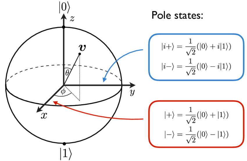
This is called as the Bloch Sphere
3. Quantum Fourier Transformation
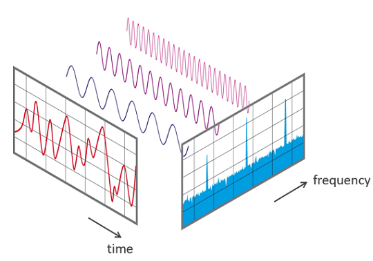
Fourier Transformation
The Fourier Transformation is transforming the wave function to frequency function. It has the following expression.
$\hat{f}(x) = \int_{-\infty}^{\infty} f(t)e^{-2\pi itx} dt$
A sequence of functions $\frac{1}{\sqrt{2\pi}}e^{ 2\pi i n} , (n$ is integer$)$ is known to be complete orthonormal basis in $L^2 ([-\pi,\pi])$. Therefore, the following expression holds.
For all $ f \in L^2([-\pi,\pi]),$ there is a unique representation $f(x) = \underset{k=-\infty}{\overset{\infty}{\sum}} \alpha_k \varphi_k(x) $ where $(\varphi_k = \frac{1}{\sqrt{2\pi}}e^{-2\pi i xk}, \alpha_k \in \mathbb{R})$
If we use the representation, then we can get a Fourier transformation as follows.
$\hat{f}(x) = \int_{-\infty}^{\infty} f(t)e^{-2\pi itx} dt$
$=\int_{-\infty}^{\infty} \underset{k=-\infty}{\overset{\infty}{\sum}} \alpha_k \varphi_k(t) e^{-2\pi itx} dt$
$=\underset{k=-\infty}{\overset{\infty}{\sum}}\int_{-\infty}^{\infty} \alpha_k \frac{1}{\sqrt{2\pi}}e^{2\pi i k} e^{-2\pi itx} dt$
$=\frac{1}{\sqrt{2\pi}}\underset{k=-\infty}{\overset{\infty}{\sum}}\alpha_k\int_{-\infty}^{\infty} e^{2\pi i t(k-x)} dt$
The latter part $\delta_k(x) = \int_{-\infty}^{\infty} e^{2\pi i t(k-x)} dt$ works as Dirac-delta function as follow
$\delta_k(x) = \begin{cases} \infty \mbox{ if }k=x \ 0 \ \ \mbox{ if } k \neq {x} \end{cases}$
Therefore, we can derive the function that gives us hints about the basis function’s period and amplitude.
To use a more intuitive way, we can see the following.
$f(t) = \sum_{i=0}^{N} \eta_i (\cos(2\pi tk_i)+i\sin(2\pi tk_i))$
$\eta_i $ is amplitude and $k_i$ is period.
It means that by using the Fourier transformation, we can decompose (or analyze) target data in trigonometric functions.
If value of some output is none-zero, then the output is amplitude and the input is period
Quantum Fourier Transform
In quantum physics, because the state of the quantum before observation is a wave, it can be represented by the wave function.
Therefore, Fourier transformation in the quantum computer can be understood as analyzing the quantum state in the frequency form.
But in the actual algorithm, the Fourier transformation rather works for a different purpose.
Every n- qubits’ state can be written like below.
$\mid \psi \rangle = \underset{j=0}{\overset{2^n-1}{\sum}} a_j \mid j \rangle_n = \underset{j=0}{\overset{N}{\sum}} a_j \mid j \rangle_n$
The $\alpha_j$ is a probability amplitude and $\mid j \rangle_n$ is the basis. There are $2^n$ possible states and $\mid j \rangle_n \in R^{2^n}$
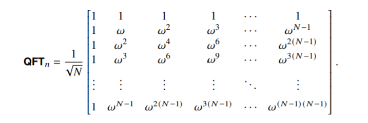
The Quantum Fourier Transformation (QFT) on it worked as below.
$QFT_n : \mid \psi \rangle = \underset{j=0}{\overset{N-1}{\sum}} a_j \mid j \rangle _n \rightarrow \underset{j=0}{\overset{N-1}{\sum}} b_j \mid j \rangle_n$
where $b_j = \frac{1}{\sqrt{N}}\underset{k=0}{\overset{N-1}{\sum}} a_k e^{\frac{2\pi jki}{N}} = \frac{1}{\sqrt{N}}\underset{k=0}{\overset{N-1}{\sum}} a_k \omega^{jk} \quad \mbox{where }\omega = e^{\frac{2\pi i}{N}}$
Because this calculation only contains linear transformation, it can be represented as matrix.이러한 연산은 인풋의 선형 변환으로만 이루어져 있으므로 행렬을 통해서 표현할 수 있다.
The result of QFT onto n-qubits is below.
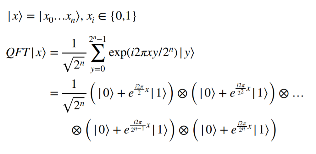
Let’s see the transformation above. The probabilities of each state are unchanged but the amplitudes of them are changed. Concretely, the n-qubit phase is $2 \pi i \frac{x}{2^n}$ , thus it rotates by $\phi = \frac{x}{2^n}$. In the Bloch Sphere, it rotates by $\frac{x}{2^n}$ with the z- axis fixing z=0.
We can express them in the circuit below. $CR_k $ gate is controlled $Z^{1/K}$ gate which rotate by $180/2^{k}$ with z-axis
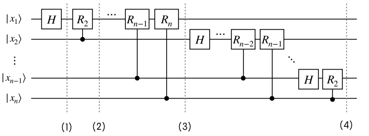
That is, we can assign each qubit to binary angles.
By using the Quantum Fourier Transformation, we can generate various algorithms. In the next posting, we’ll see these algorithms.
Sutor, R. (2019). Dancing With Qubits. Birmingham,UK:Packt
Bernhardt, C. (2019). Quantum computing for everyone. Boston, Massachusetts:The MIT Press