
Chapter 2. Quantum Gate and Basic Circuit
1. Quantum Gate
Boolean Function which was invented by George Boole, is a function that takes logical values True or False as input and returns other logical values as output.
By replacing the logical value True and false to 1 and 0 respectively, the boolean algebra can be used in computers. And by weaving the functions meticulously, we can solve much more complicated computational problems.
This logical function used at basic design of the algorithm is called Logical Gate. There are main examples of the gates; And,Or,Not,Nand etc.
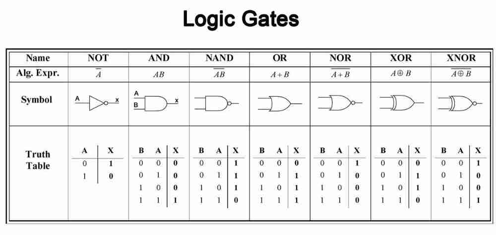
Like the classical computer, the quantum computer also uses similar gates for qubits.
As mentioned in a previous posting, the qubits in the quantum computer are represented by 2-dimensional vectors. Therefore the gate have to work as taking n-dimensional vector and returning n-dimensional vector. The operator in mathematics doing this role is matrix, so the relation between bits and gates can be replaced by vector and matrix at the quantum computer.
There is a quantum gate named Pauli Transformation Gate, Rotation Gate and Hadamard Gate which takes one qubit and returns one qubit. For gates which take two qubits and return two qubits, there are CNOT gates and SWAP gates. There are tremendous examples of the gates but the most important gates are above. Let’s figure them out.
1. Single Qubit Gates
Pauli Transformation Gates
Pauli Transformation Gates are four kind of gates which take one qubit and are $2\times 2$ matrix
$I = \left[ \begin{array}{cc} \ 1 & 0 \\ 0 & 1 \end{array} \right], X = \left[ \begin{array}{cc} \ 0 & 1 \\ 1 & 0 \end{array} \right] , Y = \left[ \begin{array}{cc} \ 0 & -i \\ i & 0 \end{array} \right] , Z = \left[ \begin{array}{cc} \ 1 & 0 \\ 0 & -1 \end{array} \right]$
For any qubit $\mid \psi \rangle = \alpha \mid 0 \rangle + \beta \mid 1 \rangle$, the qubit is transformed as follows.
-
$I\mid \psi \rangle = \alpha \mid 0 \rangle + \beta \mid 1 \rangle$
-
$X \mid \psi \rangle = \beta \mid 0 \rangle + \alpha \mid 1 \rangle$
-
$Y\mid \psi \rangle = -\beta i \mid 0 \rangle +\alpha i \mid 1 \rangle $
-
$Z \mid \psi \rangle = \alpha \mid 0 \rangle -\beta \mid 1 \rangle$
Let’s see how each probability changes. For the X gate, the amplitudes of 0 and 1 are changed each other and for the Z gate, the sign of the amplitude of 1 is charged but its magnitude is not changed. For the Y gate, we can observe that both the phases and amplitudes are changed.
We can understand X gate somehow, but it is hard to understand Y and Z intuitively. Fortunately, we can understand them easily by using Bloch Sphere.
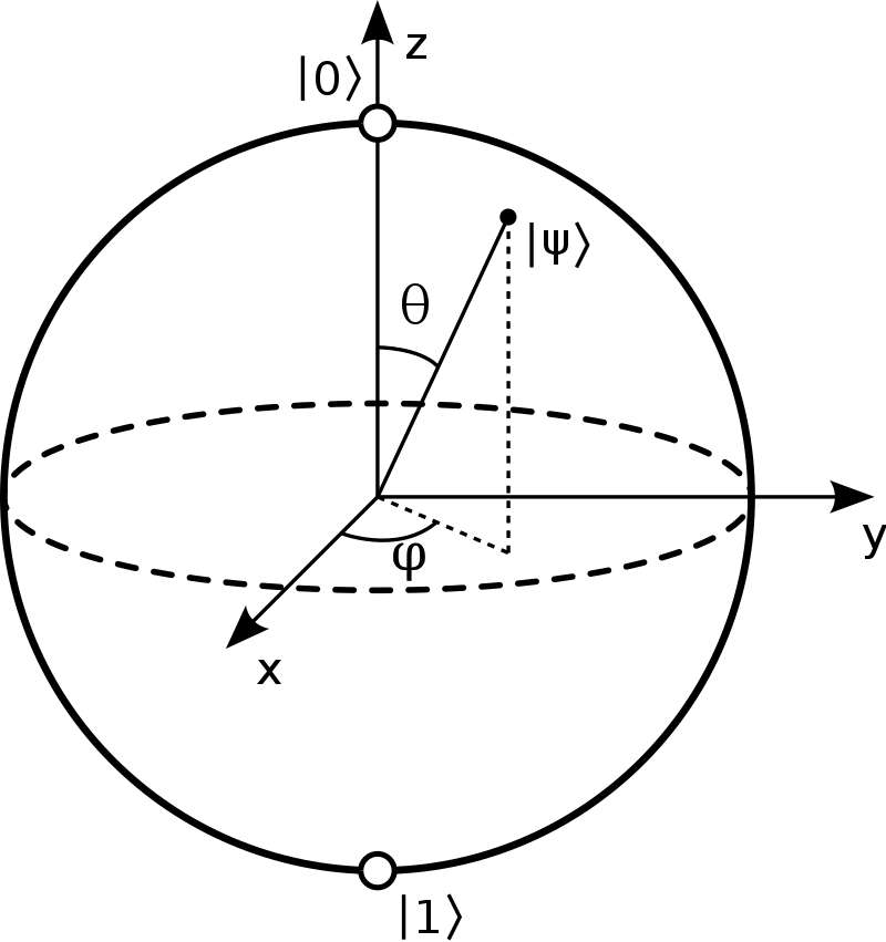
By substituting the vectors and results above, we can know that each matrix works as a rotating operator which rotates each vector as 180’ degree along with each axis.
For the rotation along the Z-axis, the vertical direction is not changed. Thus the probabilities are unchanged but the amplitudes in it turn opposite.
Like them, the pauli gates make qubit’s state opposite along each axis.
Hadamard Gate
Hadamard Gate is an essential gate of the quantum computer and expressed as below.
$H = \frac{\sqrt 2}{2}\left[ \begin{array}{cc} \ 1 & 1 \\ 1 & -1 \end{array} \right]$
This gate transforms the fixed state as $\mid 0 \rangle$ or $\mid 1 \rangle$ to superposition state of 50:50. Its results is follow
-
$H\mid 0 \rangle = \frac{\sqrt 2}{2}\mid 0 \rangle + \frac{\sqrt 2}{2}\mid 1 \rangle = \mid + \rangle$
-
$H \mid 1 \rangle = \frac{\sqrt 2}{2}\mid 0 \rangle - \frac{\sqrt 2}{2} \mid 1 \rangle = \mid - \rangle$
Or, it can be interpreted as 90’ degree rotation along the Y-axis.
For the other gates, there is a $\theta$- Rotation Gate which rotates the state $\theta$’ degree with each axis.
2. Two and Three Qubit Gates
To represent two or more qubits, the quantum computers use Tensor Product which accounts for every possible case.
$\mid \Psi_1 \rangle \otimes \mid \Psi_2 \rangle = \left[ \begin{array}{c} \ \psi_{11} \\ \psi_{12} \end{array} \right] \otimes \left[ \begin{array}{c} \ \psi_{21} \\ \psi_{22} \end{array} \right] \\ \qquad \qquad \quad =\left[ \begin{array}{c} \ \psi_{11}\left[ \begin{array}{c} \ \psi_{21} \\ \psi_{22} \end{array} \right] \\ \psi_{12}\left[ \begin{array}{c} \ \psi_{21} \\ \psi_{22} \end{array} \right] \end{array} \right]$
For general linear algebra, Dot product is the main operator. So if the operator between subjects is emitted, then it is regarded as a Dot product. However, in quantum physics, the Tensor product is the main operator. So if the operator between subjects is emitted, then it is regarded as a Tensor product like below.
$\mid \Psi_1\rangle \otimes \mid \Psi_2\rangle = \mid \Psi_1 \rangle \mid \Psi_2 \rangle = \mid \Psi_1 \Psi_2\rangle$
With this notation, let’s see 2- qubit gates
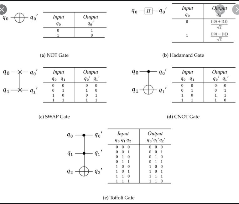
CNOT Gate
CNOT gate is abbreviation of Controlled Not Gate and it can be called as CX gate because the X gate is equal with not gate
It takes two inputs and if the first input is 1, then it applies an X gate to the second input and if the first input is 0, then it returns the second input as it is.
The matrix form of the gate is below.
$CX = \left[ \begin{array}{cccc} \ 1 & 0 & 0 & 0 \\ 0 & 1 & 0 & 0 \\ 0 & 0 & 0 & 1 \\ 0 & 0 & 1& 0 \end{array} \right] $
For this gate, the name Controlled X qubit is named because the first input controls the second input. Like the CX gate, there are gates in the quantum computer that one input controls the other qubit. Therefore, there are CZ or CY gates too.
One of the important usages of the CX gates is that it can make a bell’s circuit.
SWAP Gate
Swap Gate literally interchanges states of two qubits with each other. The matrix form of the gate is below.
$SWAP = \left[ \begin{array}{cccc} \ 1 & 0 & 0 & 0 \\ 0 & 0 & 1 & 0 \\ 0 & 1 & 0 & 0 \\ 0 & 0 & 0 & 1 \end{array} \right] $
Toffoli Gate
Toffoli Gate is also called CCNOT gate or CCX gate. It takes three inputs and returns three outputs.
It apply NOT gate to the third input when all of the first and second inputs are one
Fredkin Gate
Fredkin Gate is also called CSWAP gate. It takes three inputs and returns three outputs.
It apply SWAP gate to the second and third qubit when the first input is one
Like above, the gates can be made with these ways. By combining rotation, swap and control, we can make a lot of gates.
2. Basic of Quantum Circuit
As a combination of the above gates, we can make some circuits called Quantum Circuit which take specific roles.
IBM provides several quantum computers as open source and lets people use them with a Python package called Qiskit.
Even though Google and Microsoft also makes the quantum computer language called as Q# or circQ, but the IBM Qiskit becomes dominant role in the quantum computer and canon,
In the qiskit, the quantum circuits are depicted as figure below
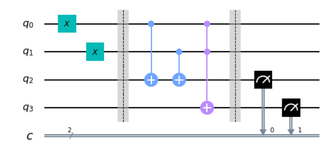
Inputs move into the left side of the circuit and they flow to the right and pass through the gates. For some hardware reasons, all of the input qubits are in the $\mid 0 \rangle$ state. The rightmost gates with the instrument panel are measuring the input qubits.
For the single qubit gates. The English character written above directly represents the gate. That is, X means X gate. For the two qubit gates, they are represented below.
Therefore, we can build custom circuits by using them.
The circuits can do some realistic action. But to understand the quantum machine learning algorithm, it is inevitable to use complex numbers. For example, in quantum machine learning, there are circuits named as quantum fourier transformation or variational quantum circuits in which the phase and complex number do essential roles.
Therefore, let’s see them after understanding the basics of complex numbers in a later posting. Instead, let’s see a more simple circuit which can be dealt with only real numbers.
Bell’s Circuit
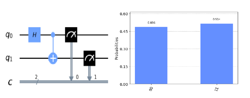
Bell’s circuit is a very simple circuit which consists of just hadamard gate and cnot gate.
Let’s see the result of this circuit mathematically.
- Input: $\mid 00 \rangle$
- Apply H gate : $(H\mid0 \rangle) \otimes \mid 0 \rangle = \frac{1}{\sqrt{2}}(\mid 0 \rangle + \mid 1 \rangle) \otimes \mid 0 \rangle$
- Apply CNOT gate: $\frac{1}{\sqrt 2} (\mid 00 \rangle +\mid 11 \rangle)$
If the input qubit is fixed 00 state, then the bell’s circuit returns the state that if one qubit is zero then the other qubit is zero and if one qubit is one then the other qubit is one. This can be called a totally entangled state.
Now, let’s see what can be done when the input qubit is fixed in 01 state by applying X gate to the second qubit.
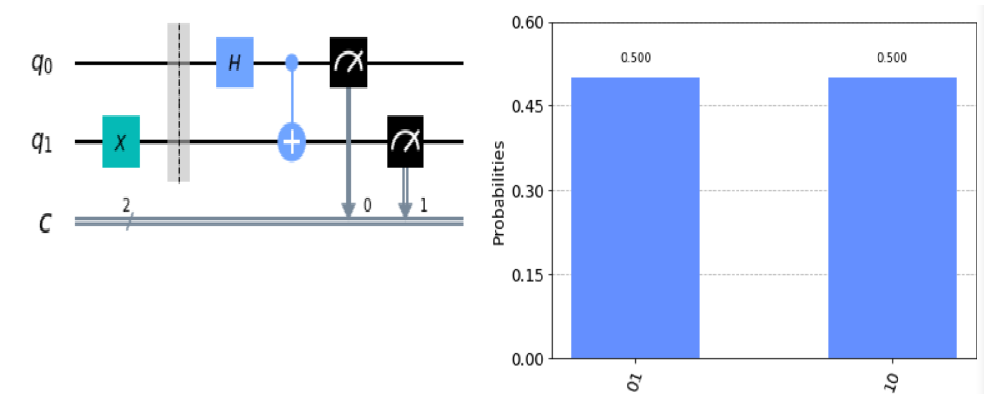
The result is similar but in this time, the state become if the one qubit is zero then the other qubit is one and if the one qubit is one then the other qubit is zero
As we see above, the bell’s circuit is used to make two perfectly entangled qubits. Particularly, the four results of the bell’s circuit are called bell’s states.
By using similar logic, we can make three or more qubits which are perfectly entangled.
We have seen the basic components of the quantum computer. But as mentioned above, to make more complicated circuits, we have to understand the phase and fourier transformation. Therefore, in the next posting, we’ll see this part.
Sutor, R. (2019). Dancing With Qubits. Birmingham,UK:Packt
Bernhardt, C. (2019). Quantum computing for everyone. Boston, Massachusetts:The MIT Press