
0. What is Qiskit?
Qiskit is a python package developed by IBM. It is an open source quantum computing framework which is designed to approach the quantum computer using a cloud system and constructing the quantum circuits.
The research of quantum computing is done with the process that researchers send the pre-designed circuits to IBM and IBM operates the received circuit with their quantum computer. Qiskit is the framework to control these processes.
Qiskit contains various abilities but this posting focuses on construction of quantum circuits. We’re gonna see 1. start the qiskit, 2. design circuit, 3. request experiments and 4. get the results
In actuality, Qiskit provides a lot better tutorials than this posting. Check it https://qiskit.org/documentation/getting_started.html
1. Starting Qiskit
Qiskit is best working with the Jupyter notebook of Anaconda. Therefore, we have to install the notebook at https://www.anaconda.com/products/individual
Qiskit is distributed with the name “qiskit”. So it can be easily installed by typing “pip install qiskit” in the prompt like below.
pip install qiskit
pip install qiskit[visualization]
Now, we can call qiskit by “import qiskit” in the jupyter notebook
To approach real quantum computers, we have to get authorities at the IBMQ. With the following link(https://quantum-computing.ibm.com/) , sign in IBMQ.
Let’s copy API token in the red rectangular in the below figure.
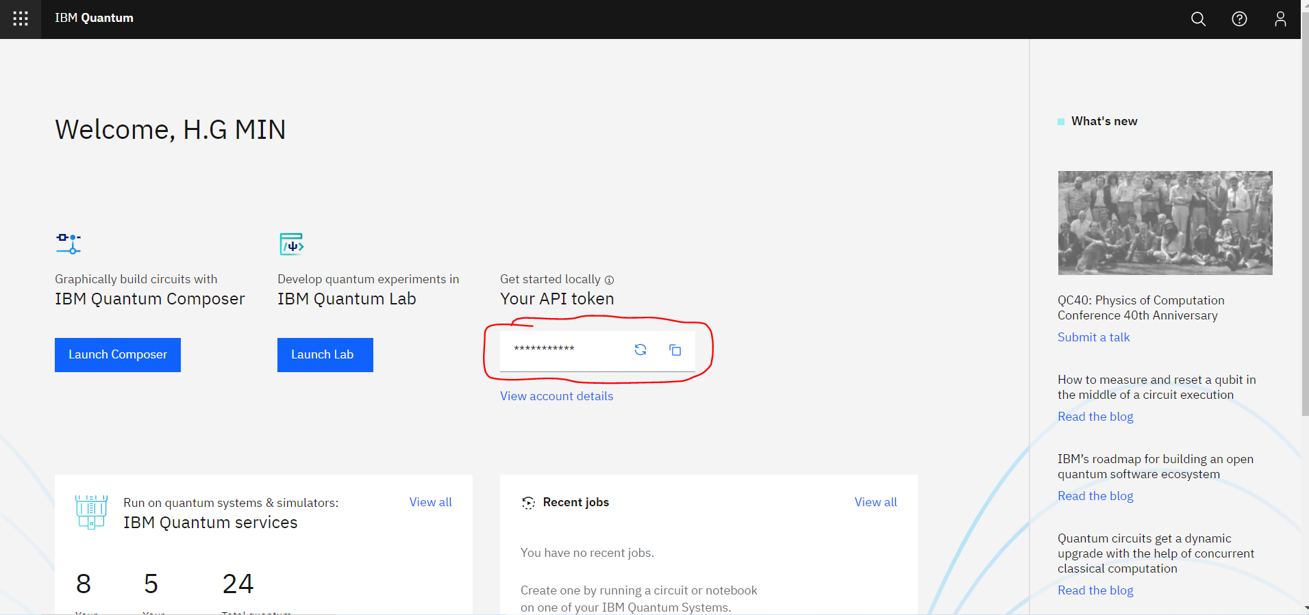
The copied code can be saved in the local and we can emit the process next time.
from qiskit import IBMQ
IBMQ.save_account('MY_API_TOKEN')
# copied code have to be typed at MY_API_TOKEN
2. Designing Circuit
A. Importing Qiskit
To import qiskit, we need to type the following command.
from qiskit import QuantumCircuit, execute, Aer
B. Making circuit instance
Quantum circuits are not that complex. Therefore, we can save them in one instance.
The command to build an instance to store the circuit is below.
circ = QuantumCircuit(n_input,n_output)
-
n_input represents the number of input qubits and n_output represents the number of output qubit
-
If there is only one number in the argument, it automatically set the input and output with same number
C. Adding measure
We can add the measurement with the below command.
circ.measure(i,j)
-
Character i means index of qubit. It start with zero
-
Character j represent the location of the bits which store the measurement result of i qubits
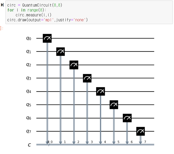
ㄹ. Visualizing Circuit
We can visualize them with the following command.
circ.draw(output='mpl',justify='none')
-
It visualizes circ instances.
-
By adding “output=’mpl’”, it shows more fancy plot by using the package “matplotlib”
ex)
The result of the above command is below.
D. Testing circuit
We can use a real quantum computer or use a simulator. The relevant command is below.
result =execute(circ,Aer.get_backend('qasm_simulator')).result()
- Inject designed circuit in the “circ”
- By using Aer.get_backend(), we can assign a computer or simulator.
- There are simulator named as “qasm_simulator” or “statevectorsimulator”
- By using “imbq.jobs”, we can use real quantum computer of IBM
- If there is no additional options, they iterate 1024 times
E. Adding gates
We can add other gates in the same way like adding measurement. It is added from the front of the circuits.
# Pauli Gate : Apply to n_q qubit
circ.id(n_q)
circ.x(n_q)
circ.y(n_q)
circ.z(n_q)

# Cliford Gate : Apply to n_q qubit
circ.h(n_q)
circ.s(n_q)
circ.sdg(n_q)
circ.t(n_q)
circ.tdg(n_q)
circ.rx(n_q)
circ.ry(n_q)
circ.rz(n_q)

# Control and Swap Gate : Apply to n_q1 and n_q2 qubit
circ.cx(n_q1,n_q2)
circ.cy(n_q1,n_q2)
circ.cz(n_q1,n_q2)
circ.ch(n_q1,n_q2)
circ.swap(n_q1,n_q2)

# Tripple Gate : Apply to n_q1,n_q2 and n_q3
circ.ccx(n_q1,n_q2,n_q3)
circ.cswap(n_q1,n_q2,n_q3)

# Special Gate
circ.measure(n_q)
circ.reset(n_q)
circ.x(n_q).c_if(n_c,0)

# Barrier
circ.barrier()
F. Visualizing
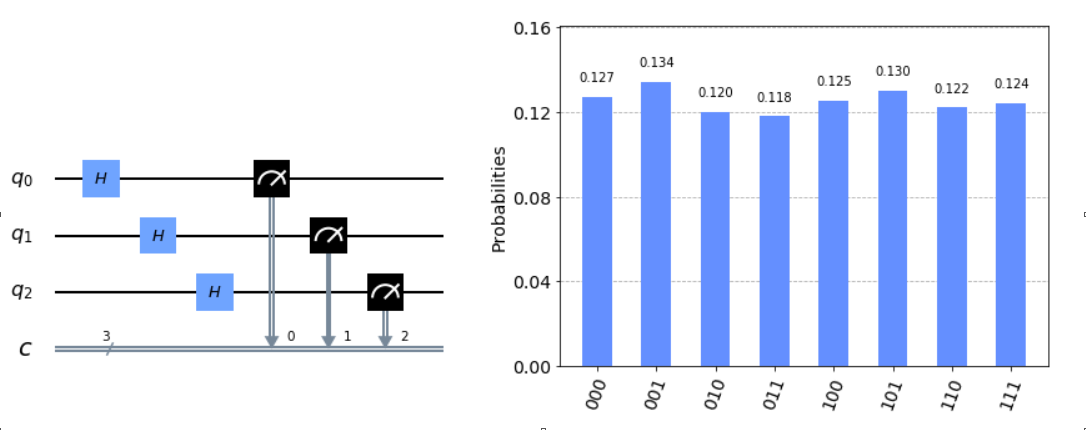
The results of the quantum algorithm are the results of 1024 shots as usual. So for the simple algorithm, histograms are working well.
from qiskit.visualization import plot_histogram
counts  = result.get_counts()
plot_histogram(counts)
Moreover, we can visualize two experiments at once.
legend = ['First execution', 'Second execution']
plot_histogram([counts, second_counts], legend=legend)
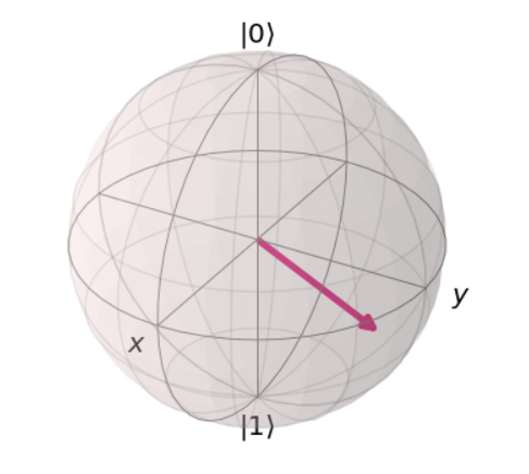
Finally, we can draw the Bloch sphere like below.
from math import sqrt, pi
from qiskit_textbook.widgets import plot_bloch_vector_spherical
coords = [3*pi/4,3*pi/4,1] # [Theta, Phi, Radius]
plot_bloch_vector_spherical(coords) # Bloch Vector with spherical coordinates
Sutor, R. (2019). Dancing With Qubits. Birmingham,UK:Packt
Bernhardt, C. (2019). Quantum computing for everyone. Boston, Massachusetts:The MIT Press