
$\def\ket#1{\mid #1 \rangle}$
1. Basic of the quantum algorithms
As mentioned before, the quantum computer can make improvements compared to the classical computer due to its unique algorithm.
When implementing them, there are several Quantum routines which are frequently used and show the intuitive reasons for the quantum speedup.
In the “Schuld, M. & Petruccione, F. (2019). Supervised Learning with Quantum Comput-ers,Cham, Switzerland:Springer ‘’, they introduce three important quantum routines; Grover Search, Quantum Phase Estimation, Matrix Multiplication. In addition to these routines, I’ll introduce inner product measurement methods at a later posting.
First of all, let’s see Grover’s searching algorithm.
a. Oracle
Oracle is a kind of function and its name is derived from the divine message of ancient Greek myth.
Oracle can take any value such as numbers or characters as inputs but only return logical values 0 or 1 as outputs. When dealing with Oracle, we cannot know the exact process of the oracle. That is, the only thing we could know is just the output of them. Therefore, we can call it a Black Box model.
Moreover, computers take everything like characters or figures with one and zero. Therefore, we can generalize Oracle in the computer as follows.
Oracle $f : {0,1}^n \rightarrow {0,1}$
Every operation in the quantum computer is done by Unitary Matrix. Therefore, the Oracle functions are made by the unitary matrix too. They are made like below.
$U_f(\ket x) = \begin{cases} -\ket x \quad \mbox{ if } f(\ket x) = 1 \\ \ket x \qquad \mbox{ if } f(\ket x) = 0 \end{cases}$
This oracle just flips the amplitudes of the result. If the result is one, then it turns it negative direction and if the result is zero, then it turns it to positive direction (unchanged)
Let’s see an example.
Imagine there are three qubits which have states like below.
$\ket \psi = a_1\ket{000} + a_2 \ket{001} + a_3 \ket{010} + a_4 \ket{100} + a_5 \ket{011} + a_6 \ket{101} + a_7 \ket{110} + a_8 \ket{111}$
If the oracle returns 1 on $\ket{010}$ and returns 0 on the other cases, then the unitary matrix would be like below.
$\ket \psi = a_1\ket{000} + a_2 \ket{001} - a_3 \ket{010} + a_4 \ket{100} + a_5 \ket{011} + a_6 \ket{101} + a_7 \ket{110} + a_8 \ket{111}$
Our purpose is to find the negative qubit state with the assumption that we don’t know the location of them. Amplitude amplification can do such a thing.
b. Amplitude Amplification
Let’s think $\psi$ has a uniform superposition state which is the result of passing multiple Hadamard gates (Kronecker Gate).
$\ket \psi = \sum_{j=1}^{8} \frac{1}{\sqrt 8} \ket j$
The character “j” in this notation represents the decimal expression of the 3 units binary expression. Let’s regard 000,001,…,111 as a binary scale and transform it into decimals. Then we can get the above expression.
If we pass the qubits to $U_f$, then we can get below states
$U_f \ket \psi = \frac{1}{\sqrt 8}\ket{000} +\frac{1}{\sqrt 8} \ket{001} - \frac{1}{\sqrt 8} \ket{010} + \frac{1}{\sqrt 8}\ket{100} +\frac{1}{\sqrt 8} \ket{011} + \frac{1}{\sqrt 8} \ket{101} + \frac{1}{\sqrt 8} \ket{110} + \frac{1}{\sqrt 8} \ket{111}$
At this time, the probabilities of each state are all the same. However, by applying some operation, we can change the probabilities which is called as Amplitude Amplification
There are various techniques to do it, but most famous one is Inversion about the mean technique
If we take the inversion about mean to eight amplitudes, then the amplitude of $\ket{010}$ who has the only negative amplitudes increases and the amplitudes of the other ones decrease. Let’s see the figure below.
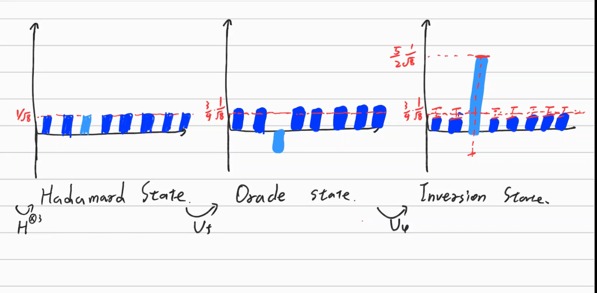
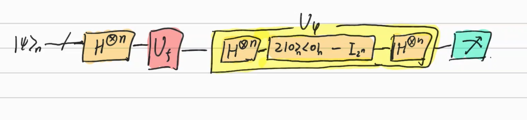
The operator $U_{\psi}$ of inversion about the mean is below.
$U_\psi = 2\ket \psi \langle \psi \mid - I_{2^n} \quad (\ket \psi \mbox{ is hadamard state}) \\ \quad = H^{\otimes n} (\mid 0 \rangle^{\otimes n} \langle 0 \mid ^{\otimes n} - I^{\otimes n})H^{\otimes n}$
This is called as Grover diffusion operator
The operator gives us some intuition in that it is similar to the projection matrix.
If we use them, then we can get more practical algorithms.
2. Grover’s Searching Algorithm
The searching algorithm of the classical computer
The amplitude amplification is used in various regions. One of them is searching. First of all, let’s see the searching algorithm in the classical computer.
Imagine there are 100 boxes and each box contains one type of the various chocolates. One of the boxes contains a mint chocolate and I want to find the box and eat it. Assuming the process of opening the boxes one by one, the case which takes the shortest steps is finding the mint chocolate in the first box and the case which takes the longest steps is not finding the chocolate until opening the 99th box.
Therefore, it takes at least one step and at most 99 steps. We can say that if the set of the box is S and the size of the set is n, then the time complexity function of the classical search is O(n). If we regard opening the box and checking the types of the chocolates as oracle, then we can interpret them as repeating the Oracle n times.
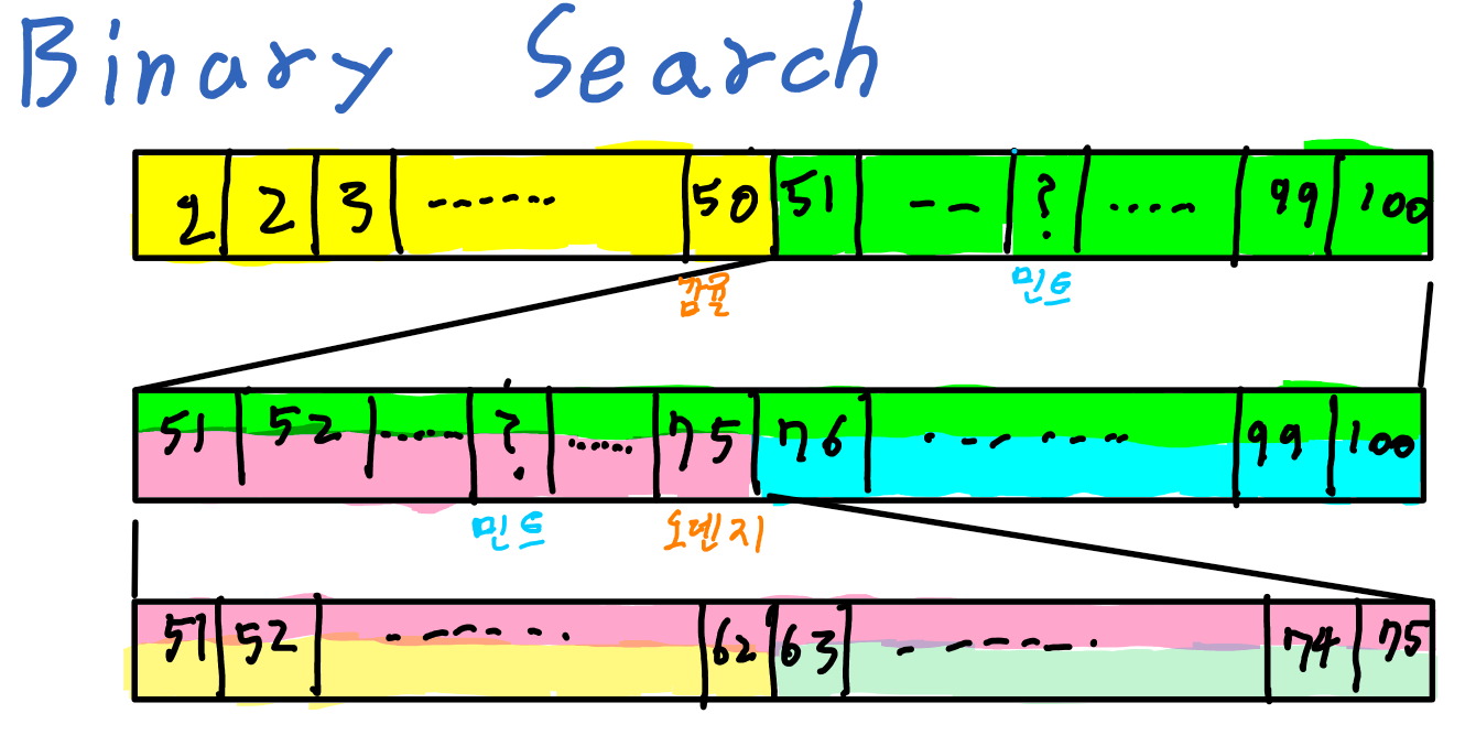
If there is additional information about the set, then we can find it faster. For example, let’s assume that the boxes are sorted based on the order of the name of the chocolates. Assume that we open the 50th box, check the name of the chocolate and figure out it is Orange. Then we could know that the mint chocolate is contained in one of the 1~50th boxes.
For the next step, if we open the 25th box and the chocolate in it is Hazelnut, then we can know that the mint chocolate will be in the 25~50th box. This way, we can search the location of the specific value more efficiently. This way is called Binary Search. And because it takes steps as $m(;m-1< \log_2 n < m)$, its time complexity function is $O(\log n)$. Therefore, it makes some exponential improvement. However, the binary search needs the premise that the set has to be sorted.
Meanwhile, Grover’s searching algorithm in the quantum computer has $O(\sqrt{n})$ as a time complexity function. It means that Grover’s algorithm shows Quadratic Improvement. Let’s figure it out.
Grover’s Algorithm
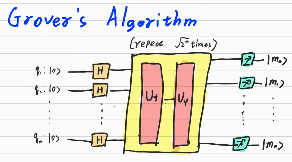
The process of the Grover’s algorithm is like below.
- Check the size N of the set S and find n such that $2^{n-1} \leq N\leq2^n$
- Construct or derive the oracle matrix $U_f$ which works to reverse the amplitudes of the basis ket. This can be defined or found in the database.
- Measure the state after applying $U_f U_{\psi}$ with $\sqrt{2^n}$ times. The measured state means the location of the target ket
The classical searching algorithm applies the Oracle to each box and the Grover’s algorithm applies the Oracle to entire boxes at once.
It is based on the amplitude amplification and it has to be applied multiple times. By applying multiple times, the amplification’s performance can be enhanced and it makes the gap between the probabilities increasing.
Obviously, there are errors to return non-target kets, and this error probability is $O(\frac{1}{N})$
3. Deutsch - Jozsa Algorithm
Deutsch’s algorithm is suggested at an early age of the quantum algorithm. Even though its practical usage is not that high, the algorithm is the first example that the quantum algorithm can show astronomical speedup compared to the classical computer. The Deutsch-Jozsa Algorithm is a multiple version of the Deutsch algorithm.
The target problem of the algorithm is below.
Whether the function $f:{0,1}^n \rightarrow {0,1}$ is a balanced function or a constant function?
The balanced function is a function where half of the inputs are mapped to zero and the other half of the input are mapped to one. The constant function maps every input to either one or zero. These too are kinds of the Oracle.
In the classical computer checking the $2^n$ inputs, the best case is returning zero at the first step and returning one at the second step. In these cases, we can directly know that they are not constant functions. In the worst case, the returned values until $2^{n-1}$ are all the same values. In this case, we can determine them at $2^{n-1}+1$ step. Moreover, if the function is constant, then we have to check until $2^{n-1}+1$. However, the time complexity of the Deutsch’s algorithm is $O(1)$
Hadamard Math
This dominant efficiency comes from the superposition of the quantum states using the hadamard gate
$H \ket 0 = \frac{\sqrt 2}{2}(\ket 0 + \ket 1)$
$H \ket 1 = \frac{\sqrt 2}{2}(\ket 0 - \ket 1)$
We can rewrite them as follow for $u \in {0,1}$
$H \ket u = \frac{\sqrt 2}{2} (\ket 0 +(-1)^u \ket 1) = \frac{\sqrt 2}{2} \underset{v \in {0,1}}{\sum} (-1)^{uv} \ket v$
Multiplying -1 does not affect the probabilities but affects the amplitudes. Physicists said this as Phase Change.
We can generalize above result as follow
$H^{\otimes n} \ket u = H\ket u_1 \otimes H \ket u_2 \otimes … \otimes H \ket u_n= \frac{1}{\sqrt{2^n}} \underset{v \in {0,1}^n}{\sum} (-1)^{u\cdot v} \ket v$
In the Deutsch - Jozsa Algorithm, we use $\ket u = \ket{00…001}$ with n+1 qubits. In this case, because of $u \cdot v = v_{n+1}$, we can write them as follows.
$H^{\otimes n +1} \ket {00…01} = \frac{1}{\sqrt{2^{n+1}}} \underset{v \in {0,1}^{n+1}}{\sum} (-1)^{v_{n+1}} \ket v $
$= H^{\otimes n} \ket 0 ^{\otimes n} \otimes H \ket 1$
Deutsch - Jozsa Algorithm
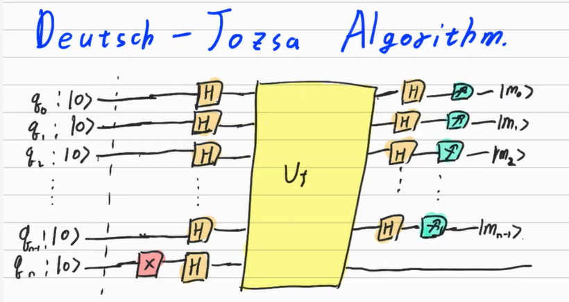
Left side part of the $U_f$ describes the above circumstance. The $U_f$ work as follow
$U_f (\ket x ^{\otimes n} \otimes \ket y) = \ket x ^{\otimes n} \otimes \ket {y \oplus f(x)}$
Each of the $\ket x^{\otimes n}$ and $\ket y$ is as follows.
$\ket x^{\otimes n} = H^{\otimes n} \ket 0 ^{\otimes n} = \frac{1}{\sqrt {2^n}}\underset{x \in {0,1}^n}{\sum} (-1)^{f(x)} \ket x$
$\ket{y} = H \ket 1 = \frac{1}{\sqrt 2} (\ket 0 - \ket 1)$
If we apply $U_f$, then we can get follow result
$U_f (\ket x ^{\otimes n} \otimes \ket y) = ( \frac{1}{\sqrt {2^n}}\underset{x \in {0,1}^n}{\sum}\ket x) \otimes (\frac{\sqrt 2}{2} \ket{f(x)} - \frac{\sqrt 2}{2}\ket{1\oplus f(x)})$
If $f(x)$ is zero, then $(\frac{\sqrt 2}{2} \ket 0 - \frac{\sqrt 2}{2}\ket{1})$
If $f(x)$ is one, then $(\frac{\sqrt 2}{2} \ket 1- \frac{\sqrt 2}{2}\ket 0)$
We can merge the result and rewrite them
$(-1)^{f(x)}\frac{\sqrt 2}{2} (\ket 0 -\ket 1)$
The probability of the state is transferred to the former part with entanglement. So we can write it as follows.
$U_f (\ket x ^{\otimes n} \otimes \ket y) = ( \frac{1}{\sqrt {2^n}}\underset{x \in {0,1}^n}{\sum} (-1)^{f(x)} \ket x)(\frac{\sqrt 2}{2} \ket 0 -\frac{\sqrt 2}{2} \ket 1)$
The latter part is a constant. In the former part, the Oracle f(x) is contained in the form as $(-1)^{f(x)}$.
Now, let’s apply the hadamard gate again. We can use the formula of the hadamard gate mentioned above.
$H^{\otimes n}(\frac{1}{\sqrt {2^n}}\underset{x \in {0,1}^n}{\sum} (-1)^{f(x)} \ket x) = \frac{1}{2^n}\underset{x \in {0,1}^n}{\sum} (-1)^{f(x)} \underset{v \in {0,1}^n}{\sum} (-1)^{x\cdot v}\ket v$
If the f(x) is constant, then we can take it out because f(x) = c like below.
$=\frac{1}{2^n}(-1)^{f(0)} \underset{v \in {0,1}^n}{\sum} [ \underset{x \in {0,1}^n}{\sum} (-1)^{x\cdot v}]\ket v$
If $\ket v = \ket {0}^{\otimes n}$, then $\forall x, x \cdot v = 0 $ and $[ \underset{x \in {0,1}^n}{\sum} (-1)^{x\cdot v}] = 2^n$
If $\ket v \neq \ket 0^{\otimes n}$, then for the combination of x, the half of the $x \cdot v$ is zero and the half of the $x \cdot v$ is one. Therefore, $ [\underset{x \in {0,1}^n}{\sum} (-1)^{x\cdot v}] = 0$
Therefore, we can get the following result.
$H^{\otimes n}(\frac{1}{\sqrt {2^n}}\underset{x \in {0,1}^n}{\sum} (-1)^{f(x)} \ket x) = (-1)^{f(0)}\ket{0}^{\otimes n}$
If we measure them, then the result if $\ket{0}^{\otimes n}$ with 100%
If the f(x) is balanced, then it becomes as follows.
$=\frac{1}{2^n}\underset{v \in {0,1}^n}{\sum} [ \underset{x \in {0,1}^n}{\sum}(-1)^{f(x)} (-1)^{x\cdot v}]\ket v$
For the $\ket v = \ket 0^{\otimes n}$, because $(-1)^{x \cdot v} =(-1)^0=1$, we can write them as follows.
$=\frac{1}{2^n}\underset{v \in {0,1}^n}{\sum} [ \underset{x \in {0,1}^n}{\sum}(-1)^{f(x)} ]\ket v$
And because half of them is zero, so $(-1)^{f(x)} =(-1)^0 =1$, and half of them is one, so $(-1)^{f(x)} =(-1)^1 =-1$
Therefore $[ \underset{x \in {0,1}^n}{\sum} (-1)^{f(x)}] = 0$ and the probability of measuring $\ket 0 ^{\otimes n}$ is zero
To sum up, if the f(x) is constant, then the probability of measuring $\ket 0 ^{\otimes n}$ is 100% and if the f(x) is balanced, the probability of measuring $\ket 0 ^{\otimes n}$ is zero. Therefore, we can determine the property of the function with Deutsch’s algorithm
Until now, we have seen Grover’s algorithm and Deutsch’s algorithm. These two algorithms are two of the most simple algorithms and good examples to understand how the probability transfer and the amplitude amplification works.
Sutor, R. (2019). Dancing With Qubits. Birmingham,UK:Packt
Bernhardt, C. (2019). Quantum computing for everyone. Boston, Massachusetts:The MIT Press