
Chapter 1. Concepts of Quantum Computer and Qubits
0. What is a Quantum Computer?
Since the first commercial computer ENIAC developed, there have been tremendous improvements in computer technologies. For instance, experts say that the computation power of modern smartphones is one billion times stronger than ANIAC and it is hard to look for someone who doesn’t have their own smartphone.
One of the fundamental technologies of this improvement is in nano technologies used in semiconductors which make it possible to set billion parts at nail-sized chips. However, the nanotechnology of semiconductors is reaching a wall that is impossible to overcome theoretically. That is, the computer hardware reached the limit.
Nevertheless, there are plenty of subjects in the contemporary academic fields which need much higher computational power than the limit. Handling super-big data or simulating millions of combinations are examples.
Therefore, the most urgent task of human beings is developing new computers which can jump over the limit of contemporary computers. And this is quantum computers.
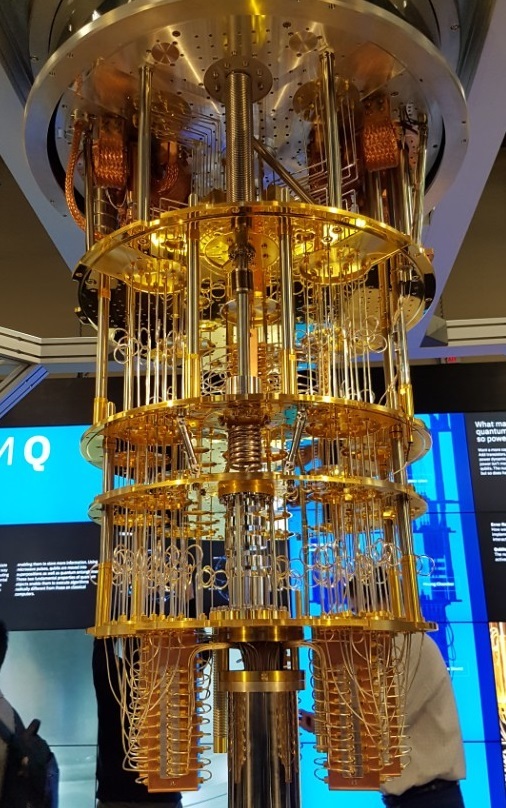
Now, several companies including Google,MS are making quantum computers and the leader of the technologies is definitely IBM. IBM already makes a 64-qubit quantum computer and experts expect that in 2023, IBM will invent a 1000-qubit quantum computer which is regarded as being able to beat super computers.
If the practical quantum computer is invented, then the paradigm of data science would be totally changed. For example, the quantum computer can accelerate the sampling methods which are regarded as less practical than the optimization methods because of its slow speed and the algorithms which are too complicated to be used in reality could also be commercially used.
To use the quantum computers, we need to know the theories and algorithms of the quantum computer. However, because the quantum computer is the combination of mathematics, physics, engineering and computer science, it is hard to know all of them.
Therefore, this series of posting focuses on understanding the basic theory of the quantum computer and only specific regions of algorithms which are relevant with data science and abandoning less interesting things like hardware or cryptography.
1. The basics of the quantum computer
The Quantum computer can solve the problems which have to take astronomical times to calculate with the classical computers. This overwhelming power is due to its software not the hardware. That is, the efficiency of the quantum computer is because it solves the problem in a totally different direction from classical computers.
Let’s see factorization. To factorize 100023, the classical computer has to divide them with prime numbers. If the remainder is 0, then the prime number is factor of 100023. It has to have at least a square root of 100023. Because the calculation needs super time, the factorization is one of the hardest problems for the classical computers.
However, the quantum computer can reduce the time dramatically by using the concepts of superposition and observing the entire result in one step. Because modern cryptography is based on factorization, the contemporary cryptosystem would be neutralized mostly.
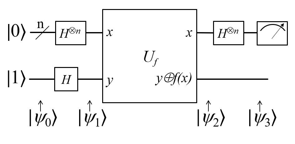
For another example, there is a Deutch’s Algorithm. If we want to know whether some specific functions are constant or balance functions, we have to see all of the results once at a time. But the quantum computer, can observe the result just one step. Therefore, the time complexity would become from n to 1.
That is, the quantum computer can work better with better algorithms. Then someone might wonder how to apply the algorithm to classical computers, but this is impossible because its base is different.
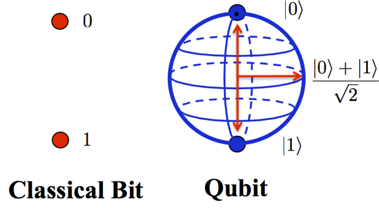
The basic unit of the classical computer is a bit which takes a value of either 1 or 0. The classical computer implements them with an electronic signal; if the signal is on, then they interpret it as 1 and if else as 0. Then it passes the bit to the gates(;transister, physically) and gets some computational results.
Meanwhile, the basic unit of the quantum computer is Qubit. This qubit contains three unique characteristics; Superposition, Measurement and Entanglement. These Three characteristics are the sources of the high efficiency of the quantum computer. Let’s figure it out.
2. Characteristics of Qubit
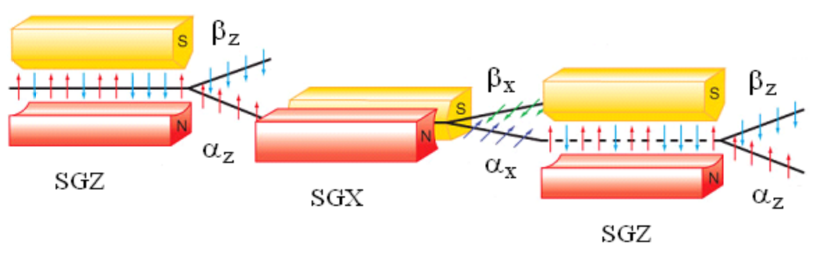
The experts usually express the bit as a switch and the qubit as a spin. This is inspired by the Stern-Gerlach experiment and we can understand almost every part of the characteristics with the experiment. Below is the depiction of the experiment, but the interpretation and details might be very different from the physicist and even might be wrong. Nevertheless, it could help the outsiders understand the concepts.
Let’s imagine a ball-shaped magnet. There is no visible discriminate line between N pole and S pole so we don’t know which direction is N pole. Let’s shoot this ball to a tunnel of measurement like below.
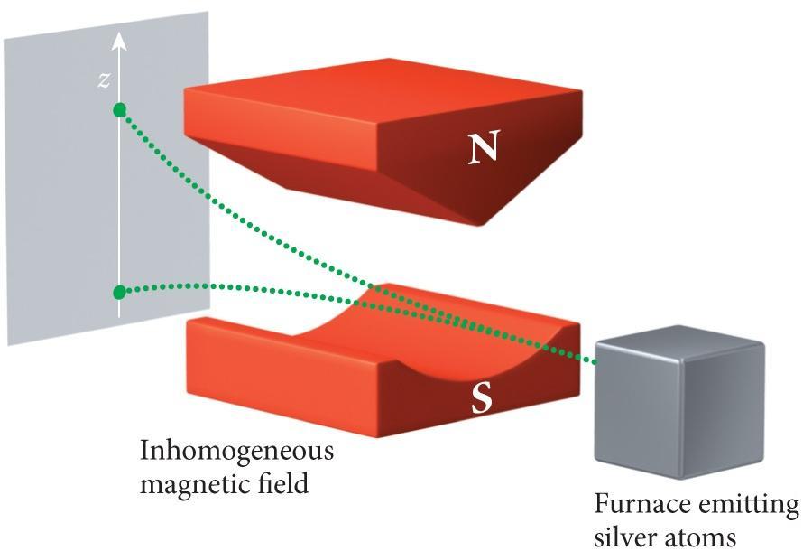
Because the N pole of the tunnel is more popped up, if the N pole of the magnetic is upside, then it will tilt downward and if the N pole is downside, then it will tilt upward
But what about if the N pole and S pole are exactly 90’ degree? Although many scientists expected that it would move horizontally, in the experiment, every magnetic tilt was either upward and downward.
Physicists thought that the direction of the magnetics might be decided before shot. They thought that because the angles might be very subtly tilted to upward or downward, like 89.99999’, they move to that side.
This explanation can be interpreted as a kind of hidden variable theory. Some variables which were unobservable and hidden determine the direction of the magnetics. This seems reasonable.
However, the Copenhagen interpretation, a canonical interpretation of quantum physics, takes a different position with this explanation.
They regard the state of the magnetic before shotten having a superposition state which means that it is pointing to upside and downside at the same time. There is no hidden variable and the direction of the magnetic is purely random.
That is, the state that can be anyone is called as superposition state. And not like the bit, qubit can be the superposition state.
As an aside, Schrödinger’s cat is to criticize this explanation. There is a cat and some toxic gas in the device which emits the gas with probability of 50%. According to the Copenhagen interpretation, the cat is dead and alive at the same time. That is, the experiment wanted to say that, in the visible real world, the explanation is totally unreasonable. Nonetheless, with some real experimental results, the Copenhagen interpretation has overtaken all other explanations and takes the canon.
Despite the superposition state being represented with uncertainty, it can be controlled. If the magnetic moves upward, then the direction of the magnet will be aligned to upward which means that if we shoot the magnetic without other touches, then we can get the result of moving upward with probability of 100%.
At this time, let’s shoot the 100% upward magnetic to the tunnel spinned by 90’ degree. In this case, we can get the magnetic which tilts downward with 50% and upward 50%.
This means that with the measurement itself, we can influence the direction of the magnetic and change the state from superposition state to non-superposition state and vice versa.
This implies two things; 1. The measurement itself affects the state of the quantum and 2. According to the direction of the measurement, we can see the state differently.
How can we make a computer with this magnet?
The definition of the quantum is something that has a physical state which can be measured discreetly. However, the physicist proved that literally everything in the world is discrete, not continuous.
Therefore, the quantum is just something that could be measured. That is, power, speed,mass everything is quantum and magnetic in the above experiment is also quantum.
If we use the similar substances which have similar properties with above magnetics and represent upward as 0 and downward as 1, then we can express the classical bit with quantum.
However, the difference between this representation and the classical bit is that it can show superpositions of 0 and 1. This is a qubit; the basic unit of the quantum computer.
Of course, because the qubit can represent 1 and 0 with 100%, they can replace the bit too. Therefore, the quantum computer can do all of the things that the classical computer can do
Finally, let find out last important characteristic of the quantum;Entanglement
Think about two bits in the classical computer. Two bits means two switches. Turning on one of the switches would not affect the other switch. That means two bit move independently.
However, the quantum computer can change one qubit by changing the other qubit. For example, let’s split a magnet and make it two. This process preserves the direction of each splitted magnet. Without changing the direction, let’s shoot one magnet to the other side of the earth. At this time, if we observe the N pole of our magnetic field pointing upwards, then we can directly know the direction of other magnetic fields on the other side of the earth.
This kind of phenomenon is called as Entanglement and by using it, we can solve various mathematical problems naturally.
This example is the most simple one and the quantum computer can make diverse types of entanglement.
Let’s summarize above.
- Quantum physics is dealing with the microworld where the Measurement itself affect the state of the subjects
- In this time, the unmeasured state is interpreted as a Superposition of several states
- In the quantum world, one quantum can be directly connected with other quantum and we called it as Entanglement.
Consequently, we can say the quantum computer is a computer using these three characteristics of the quantum world
3. Mathematical Representation of Quantum
Until this line, we can understand the basic concepts of quantum computers somehow. However, we cannot imagine concretely how these concepts could be connected with mathematical algorithms. By using the Linear Algebra, we can beautifully connect the concept of quantum and mathematical world
The qubit and algorithm of the quantum computer can be perfectly represented with linear algebra. In quantum physics, they usually use Bracket notation which is called Dirac’s notation.
One qubit can be expressed as follow

$\mid \Psi \rangle = \left[ \begin{array}{c} \ \psi_1 \\ \psi_2\end{array} \right] ;(\psi_1^2 + \psi_2^2 = 1) $
In other words, we represent the direction(;state) of the qubit with a unit vector in 2-dimensional space.
Then, someone might think that by expressing [0,1] as 0 and [0,-1] as 1, we can combine a 2-dimensional plane and a quantum world. But, unfortunately, the quantum computer takes a little bit of a different approach with this one. Concretely, like below
$\mid 0 \rangle = \left[ \begin{array}{c} \ 1 \\ 0 \end{array} \right], \mid 1 \rangle = \left[ \begin{array}{c} \ 0 \\ 1 \end{array} \right]$
If we draw them in a 2-dimensional plane, then it shows a totally different way that we normally expect in the coordinate plane. Thus, let’s forget about it and think of learning a brand new plane.
How can we express the superposition state with the above notation? Let’s see below
$\mid \Psi \rangle = \left[ \begin{array}{c} \ \psi_1 \\ \psi_2\end{array} \right] = \psi_1\mid 0\rangle + \psi_2\mid 1\rangle]$
That is, we can see it as the mixed state of the state of 0 with $\psi_1$ and the state of 1 with $\psi_2$. This is called Probability Amplitude. If we take square of them, then we can calculate the probabilities of outcome from each state.
Then how about a state of 50:50 probability?
$\mid \psi \rangle = \frac{1}{\sqrt{2}} \mid 0 \rangle + \frac{1}{\sqrt{2}} \mid 1 \rangle $
If we express it above, then because the square of each amplitude is 1/2, we can say the probability is 50:50. But, let’s see other examples.
$\mid \psi \rangle = \frac{1}{\sqrt{2}} \mid 0 \rangle - \frac{1}{\sqrt{2}} \mid 1 \rangle $
In this case too, if we take a square, we can get 50:50.
In quantum computing, these two states are different states with each other. In the previous example, if we shoot the magnetic with N-upside, we can get 50:50. But if we shoot the magnetic with S-upside, then we can see the same result too.
That is, in reality, the N pole can take many directions. Therefore, we will discern these cases. And for the above states, we named them as below.
$\mid + \rangle = \frac{1}{\sqrt{2}} \mid 0 \rangle + \frac{1}{\sqrt{2}} \mid 1 \rangle $ , $\mid - \rangle = \frac{1}{\sqrt{2}} \mid 0 \rangle - \frac{1}{\sqrt{2}} \mid 1 \rangle $
These states cannot be discriminated against with a 0’ degree tunnel. But with 90’ degree tunnel, we can perfectly discriminate between two states.
Therefore, by seeing two states as different states, we can store deeper information in one qubit.
However, the reality is 3-dimension not 2-dimension. Therefore, it would be more appropriate to use a 3-dimensional vector rather than a 2-dimensional vector.
Nevertheless, we use a 2-dimensional vector by introducing complex number i. By using a complex plane, we can represent 3-dimensional space with a 2-dimensional vector. Therefore, we can again name the special representation like below.
$\mid i \rangle = \frac{1}{\sqrt{2}} \mid 0 \rangle + \frac{i}{\sqrt{2}} \mid 1 \rangle $ ,$\mid -i \rangle = \frac{1}{\sqrt{2}} \mid 0 \rangle - \frac{i}{\sqrt{2}} \mid 1 \rangle$
We can summarize the quantum state as follows.
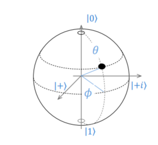
This is called as Bloch Sphere Representation
In summary, the quantum state has the generalized form as below.
$\mid \psi\rangle = \cos \theta \mid 0 \rangle + \sin \theta e^{i \phi} \mid 1 \rangle (; a^2 + b^2 =1)$
The $e^{i \phi}$ is a complex number whose norm is 1 and is called Quantum Phase specially. We will see the concept of complex numbers in the quantum computer in another posting.
Until now, we see the concepts of the quantum computer and basic unit qubit. In the next posting, we’ll see the basic quantum gates and circuits.
Sutor, R. (2019). Dancing With Qubits. Birmingham,UK:Packt
Bernhardt, C. (2019). Quantum computing for everyone. Boston, Massachusetts:The MIT Press