Full presentation
Techniques of scRNA-seq · 25 slides
Loading presentation…
This note expands my Techniques of scRNA-seq presentation dated October 2, 2026. The workflow has four stages: primary processing, quality control and preprocessing, construction of a cell landscape, and biological inference.
Each stage produces a different kind of object. Keeping track of that object helps prevent a common mistake: treating a visualization, a normalized expression matrix, and a statistical analysis as interchangeable.
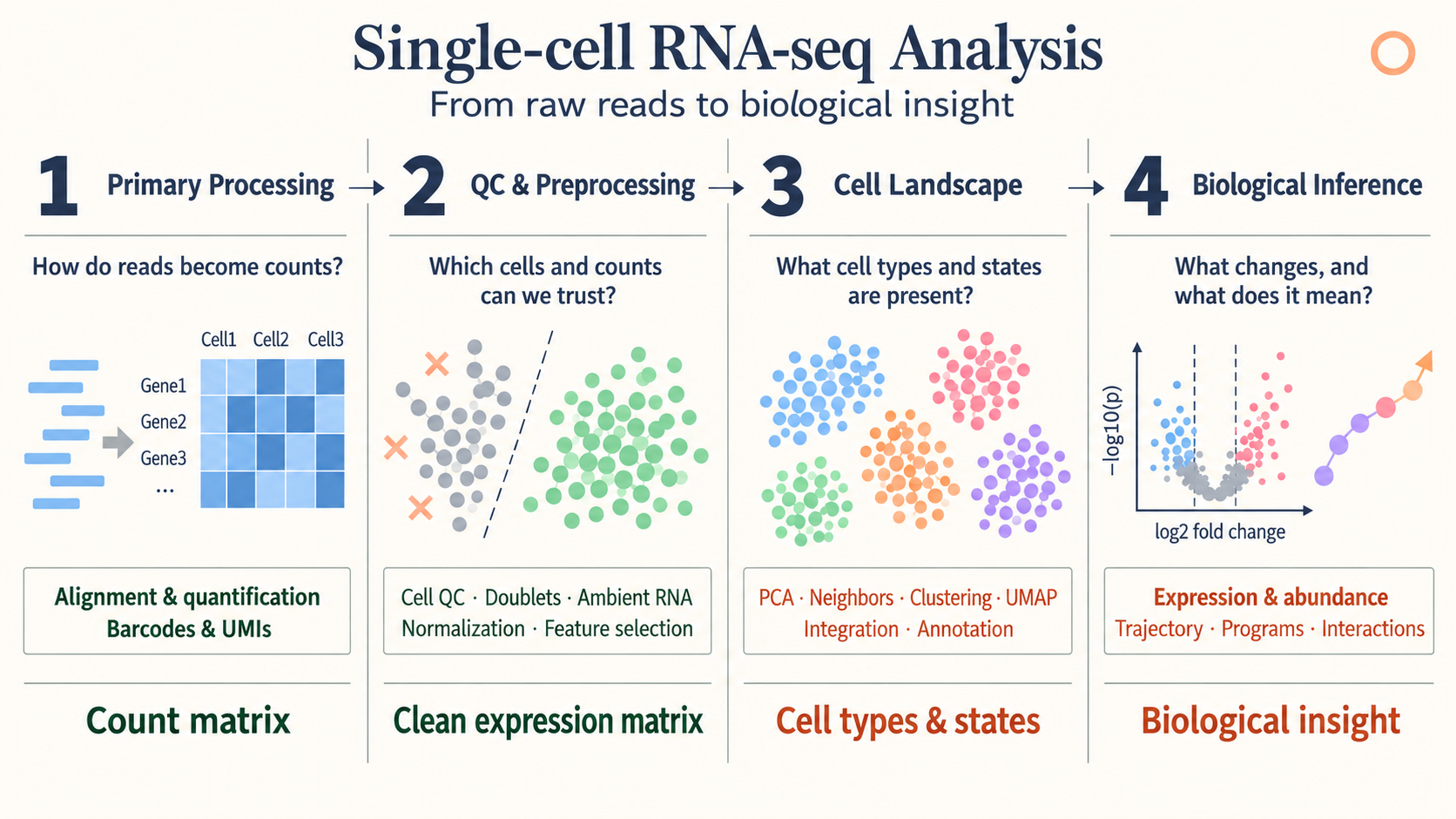 Overview from my presentation, slide 3.
1. Primary processing: FASTQ to count matrices
A transcriptomic library contains information for identifying the cell, the captured molecule, and the transcript. A cell barcode groups reads by cell. A unique molecular identifier (UMI) helps distinguish original molecules from amplification duplicates.
The conceptual processing sequence is:
- Extract and correct barcodes and UMIs.
- Assign reads to genes.
- Collapse compatible reads into molecule counts.
- Construct a gene-expression count matrix.
In a perturbation experiment, a guide library supplies a separate cell-by-guide matrix. The two matrices are connected by cell barcode. Guide assignment is an additional inference step; detecting guide reads is not identical to confirming effective perturbation.
The useful starting point for later analysis is a count matrix accompanied by sample, batch, condition, and guide metadata.
2. Quality control
Quality control asks which observations support the biological question. The presentation highlights low-count cells and genes, mitochondrial fractions, doublets, and ambient RNA.
Low counts can indicate poor capture, but thresholds depend on cell type and protocol. A high mitochondrial fraction can suggest compromised cells, yet it also varies with biological context. Doublets combine more than one cell in a barcode, while ambient RNA introduces transcripts from the surrounding suspension.
These effects are not removed by a single normalization step. Filtering decisions should be examined across samples so that one condition is not selectively depleted by a threshold.
3. Normalization and variance stabilization
Library-size normalization
A common log-normalization is
\[\widetilde x_{ig} =\log\left(1+s\frac{x_{ig}}{\sum_hx_{ih}}\right),\]where $s$ is a scale factor, often $10^4$. This adjusts the total count scale and compresses the range. It does not guarantee that every technical or biological source of variation disappears.
SCTransform and Pearson residuals
SCTransform models UMI counts with a regularized negative-binomial framework. A schematic Pearson residual is
\[r_{ig} =\frac{x_{ig}-\widehat\mu_{ig}} {\sqrt{\widehat\mu_{ig}+\widehat\mu_{ig}^{\,2}/\widehat\theta_g}}.\]The fitted mean accounts for sequencing-depth effects. The residual expresses the difference between observation and expectation relative to expected variability.
The sample-adjustment illustration in the presentation describes a model with explicit sample terms. This is not a guarantee that calling SCTransform() removes every donor or batch effect. Additional covariates and their biological meaning must be specified deliberately. See the SCTransform documentation.
DESeq2 variance-stabilizing transformation
The motivation for a variance-stabilizing transformation is that count variance depends on the mean. For a mean–variance function $v(\mu)$, the delta method gives
\[\operatorname{Var}\{h(X)\} \approx[h'(\mu)]^2v(\mu).\]Choosing
\[h'(\mu)=\frac{1}{\sqrt{v(\mu)}}\]therefore reduces mean dependence of the variance. If
\[v(\mu)=A\mu+B\mu^2,\qquad A,B>0,\]then one antiderivative is
\[h(q)=\frac{2}{\sqrt B} \operatorname{asinh}\sqrt{\frac{Bq}{A}}+C.\]The presentation uses this derivation to explain the shape of a VST. Actual DESeq2 transformations also depend on size-factor normalization and the fitted dispersion trend. A VST is useful for exploratory distances and visualization; count-based differential analysis still uses its count model.
Three similarly named operations
| Operation | Purpose | Main output |
|---|---|---|
SCTransform() |
Model depth dependence and stabilize expression variability | An assay including residual-based values |
DESeq2::vst() |
Transform count data using a mean–variance relationship | A transformed expression matrix |
FindVariableFeatures(selection.method="vst") |
Rank genes by standardized variability | A selected set of variable features |
These operations should not be treated as interchangeable because their names contain “variance” or “vst.”
4. Highly variable genes and PCA
The Seurat variable-feature procedure models the relationship between average expression and variance. It standardizes variability relative to the fitted expectation, limits extreme contributions, and ranks genes. Its role is feature selection, not a replacement for the expression matrix. See FindVariableFeatures.
PCA then represents cells with a smaller number of coordinates. For a centered matrix $X$,
\[X=UDV^\mathsf T.\]The columns of $V$ define feature directions and $UD$ supplies cell scores. Keeping the first $K$ components captures major linear variation with fewer coordinates.
The presentation uses about 50 coordinates as an example. The appropriate number depends on the data and question; a high-variance component may represent batch, cell cycle, or biology of interest.
5. Batch integration with Harmony
Harmony operates on a low-dimensional cell representation. The presentation explains it through iterative soft clustering and batch correction using a ridge-regression formulation.
Soft membership allows a cell to contribute to multiple clusters. Batch-diversity terms encourage shared biological populations to align, and correction is performed within the representation.
The resulting embedding supports neighborhood analysis. It is not a newly observed gene-count matrix. If batch and condition are completely confounded, computation alone cannot determine which difference is technical and which is biological.
For integration across different assays and feature spaces, see GLUE.
6. Neighbors, clusters, and two-dimensional maps
A neighbor graph describes local relationships among cells. Graph clustering identifies groups with relatively strong internal connectivity. UMAP and t-SNE provide low-dimensional displays of relationships.
The presentation compares their objectives:
| Method | High-dimensional relationships | Low-dimensional construction |
|---|---|---|
| t-SNE | Neighbor affinities derived from local Gaussian scales | Student-t similarities, optimized using KL divergence |
| UMAP | A locally scaled weighted neighborhood graph | A low-dimensional fuzzy graph, optimized with a cross-entropy objective |
Both optimize cell positions rather than assign biological identities. The displayed axes generally have no direct molecular units. Apparent gaps, cluster sizes, and long-range distances require care in interpretation.
Clustering is usually performed on a suitable high-dimensional or latent neighbor graph, rather than inferred solely from a two-dimensional picture.
7. Cell-type annotation with SingleR
The SingleR illustration begins with a labeled reference. It selects informative genes, compares query cells with reference profiles using correlations, and summarizes evidence for each label.
Candidate labels are refined using the features that distinguish them. Ambiguous assignments can be pruned rather than forced into a confident category.
Annotation quality depends on the reference. A population missing from the reference may receive the closest available label even when it is biologically distinct. Marker checks, sample context, and uncertainty therefore remain part of interpretation.
8. Gene expression programs
Gene programs describe coordinated expression that can cross cell-type boundaries. NMF represents each cell as a combination of nonnegative program activities; cNMF looks for programs that are reproducible across factorization runs.
A program may reflect identity, cell cycle, stress, or a response to perturbation. A cluster label and a program score answer different questions about a cell.
The cNMF and V2G2P review describes how expression programs were connected to perturbations and disease-associated genes.
9. Differential expression and differential abundance
Differential expression asks which genes change within a specified population. Differential abundance asks which populations change in frequency.
| Analysis | Response | Replication to preserve |
|---|---|---|
| Differential expression | Gene expression or counts | Independent biological samples |
| Differential abundance | Cell counts or composition | Independent biological samples |
For expression, muscat illustrates pseudobulk and sample-aware cell-level models.
For abundance, the presentation contrasts scCODA, which models cell-type composition, and Milo, which tests cell counts in overlapping graph neighborhoods. The latter can describe abundance changes without requiring all relevant states to coincide with discrete cluster boundaries.
Composition creates dependence: an increase in the relative fraction of one population changes the fractions available to others. Sampling and recovery can also influence observed proportions.
10. Trajectories with Slingshot
Slingshot uses relationships among clusters to define candidate lineage structure and fits smooth curves through cells. Cells are ordered by their position along a lineage to obtain pseudotime.
The presentation illustrates cluster connections, a selected root, fitted curves, and cell ordering. Root choice and the included populations shape the interpretation.
Pseudotime is not elapsed clock time. A trajectory through cross-sectional cells is a model of progression, and branching structure is not direct lineage-tracing evidence.
11. Cell–cell communication with CellChat
CellChat combines expression with a database of ligand–receptor interactions. It summarizes expression in proposed sender and receiver populations and evaluates potential signaling relationships.
The presentation illustrates a saturating interaction score of the form
\[S=\frac{L_AR_B}{K+L_AR_B},\]where $L_A$ and $R_B$ summarize ligand and receptor expression. This is a simplified illustration; complexes, cofactors, and method settings affect the full calculation.
Label permutations supply a comparison distribution for the observed score. A predicted interaction indicates compatibility with an expression-based signaling model. It does not directly measure ligand secretion, receptor activation, spatial contact, or causal communication.
12. Connecting the outputs
The workflow is easiest to follow by tracking what is available after each stage:
| Stage | Output | Next question |
|---|---|---|
| Primary processing | Counts and metadata | Which measurements are usable? |
| QC and normalization | Filtered counts and analysis representations | Which variation should define neighborhoods? |
| Cell landscape | Embeddings, graphs, clusters, labels | What changes across samples or conditions? |
| Biological inference | Effect estimates, programs, candidate trajectories and interactions | What evidence supports the biological interpretation? |
Raw counts, transformed matrices, and corrected embeddings each have a purpose. Preserving sample identities and documenting which representation enters each analysis makes the resulting biological claims easier to assess.
References
- Presentation source:
05.Techniques_of_scRNA.pptx, slides 1–23; presented October 2, 2026. - Seurat documentation: SCTransform and FindVariableFeatures.
- Related presentation notes: cNMF, GLUE, MAGIC, and muscat.