Full presentation
muscat · 52 slides
Loading presentation…
This note follows my presentation on Crowell et al., muscat detects subpopulation-specific state transitions from multi-sample multi-condition single-cell transcriptomics data (Nature Communications, 2020).
1. Differential state is a specific question
Several distinct questions are often grouped under single-cell differential analysis:
| Question | Comparison |
|---|---|
| Cell-type markers | One cell population versus another |
| Differential abundance (DA) | The frequency of a population across conditions |
| Differential state (DS) | Expression within a population across conditions |
A treatment may change expression in microglia without changing their abundance. Conversely, microglia may become more abundant without a strong within-population expression change.
muscat focuses on differential states in data with multiple biological samples, conditions, and cell subpopulations. It supplies an analysis and simulation framework, rather than one statistical test that replaces every existing method.
2. Cells are nested within biological samples
Cells from one donor or animal share genetic background, exposure, handling, and other sample-specific influences. They are not interchangeable with cells collected from independently sampled individuals.
If three control donors and three treated donors each contribute 1,000 cells of one type, there are six biological samples. The 6,000 cells improve observation of those samples; they do not create 6,000 independent treatment assignments.
Ignoring this structure can mistake a donor-specific difference for a reproducible condition effect. Two common strategies preserve sample information: aggregate within samples, or model sample effects at the cell level.
3. Pseudobulk aggregation
For gene $g$, sample $s$, and cell type $c$, define
\[Y_{gsc}=\sum_{i:\,\operatorname{sample}(i)=s,\, \operatorname{type}(i)=c}X_{gi}.\]This produces a gene-by-sample matrix for each cell type. A bulk count model can then compare biological replicates within that type.
An illustrative negative-binomial model is
\[Y_{gsc}\sim\operatorname{NB}(\mu_{gsc},\phi_g),\] \[\log\mu_{gsc} =\log L_{sc}+\beta_{0g} +\beta_{1g}\operatorname{condition}_s +\boldsymbol\gamma_g^\mathsf T\mathbf z_s.\]Here, $L_{sc}$ is a library-size normalization factor or effective exposure and $\mathbf z_s$ contains design covariates. For a paired experiment, the design should account for the pairing.
For count-based methods, aggregation begins with counts, not with averaged log expression or a batch-corrected embedding. Samples are not pooled across an entire condition: doing so would discard replication.
4. Cell-level mixed models
A mixed model retains individual cells and models their shared sample membership. Schematically,
\[g\{\mathbb E(X_{gis}\mid b_{gs})\} =\beta_{0g}+\beta_{1g}\operatorname{condition}_s +\boldsymbol\gamma_g^\mathsf T\mathbf z_{is}+b_{gs}.\]The random effect $b_{gs}$ captures sample-level variation. The link, distribution, and additional terms depend on the method.
This approach retains within-sample information but can be computationally demanding. Neither a mixed model nor pseudobulk aggregation can manufacture missing biological replication or resolve complete confounding in the experimental design.
5. Six method families in the presentation
The presentation organizes 16 analysis variants into six families:
| Family | Main idea | Important distinction |
|---|---|---|
| scDD | Mixture-based modeling of expression distributions | Can target changes beyond a mean shift |
| MAST | Two-part hurdle regression | Models detection and positive expression separately |
| Anderson–Darling | Comparison of empirical distributions | A distributional test, not a count GLM |
| Mixed models | Fixed effects plus sample-level random effects | Models dependence between cells from a sample |
| edgeR | Negative-binomial models with moderated dispersion and quasi-likelihood inference | Applied to sample-level pseudobulk counts in this comparison |
| limma | Linear modeling with empirical Bayes variance moderation | voom adds observation-level mean–variance weights; trend uses a mean–variance trend in moderation |
MAST should not be described simply as negative-binomial regression. Its hurdle construction separates whether expression is detected from the level of positive expression.
For nested likelihood models, the usual likelihood-ratio statistic is
\[\Lambda=2(\ell_{\text{full}}-\ell_{\text{reduced}}).\]Its chi-squared approximation requires regularity conditions and the appropriate degrees of freedom. The factor of two matters.
The model family alone also does not determine whether an analysis respects sample structure. That depends on the design and the specific implementation.
6. Simulation: more than a shift in the mean
The simulation framework learns characteristics such as library sizes and dispersion from reference data. The presentation uses the paired PBMC dataset from eight lupus patients before and after IFN-β stimulation as a reference example.
Counts are generated under several expression scenarios. The schematic distinguishes six patterns:
| Pattern | Interpretation |
|---|---|
| EE | The same unimodal distribution in both groups |
| EP | The same mixture proportions in both groups |
| DE | A shift in expression level |
| DP | Different proportions of mixture components |
| DM | Different modality, such as unimodal versus bimodal expression |
| DB | A distributional change with equal overall means in the illustrated construction |
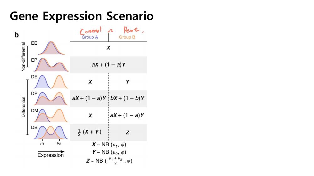 Slide 11 of my presentation; the underlying simulation schematic is from Crowell et al. (2020). EE and EP are non-differential controls.
The equal-mean example explains a fundamental limitation: a test of mean expression is not designed to detect every possible change in a distribution. A method can perform well for its target while missing a different kind of effect.
7. Reading the benchmark
The presentation evaluates discoveries using true positive rate and false discovery behavior:
\[\operatorname{TPR}=\frac{\operatorname{TP}}{\operatorname{TP}+\operatorname{FN}}, \qquad \operatorname{FDP}=\frac{\operatorname{FP}}{\max(R,1)}.\]Here, $R$ is the number of discoveries. FDR is the expectation of the false discovery proportion, rather than the false discovery proportion of one realized experiment.
High sensitivity alone is insufficient if a method also produces too many false positives. Conversely, a method may control error well but have little power for rare populations or distributional changes outside its target.
The study supports sample-aware pseudobulk and mixed-model approaches as useful strategies for multi-sample DS analysis. The choice still depends on the expression pattern, sample count, population size, computation, and desired interpretation.
The cortex application compares vehicle- and LPS-treated mice, asking which subpopulations respond transcriptionally. This returns to the main biological question: a condition can induce different responses in different cell types.
8. Implications for perturbation studies
The same design questions arise in CROP-seq and other perturbation experiments. One must identify what was independently assigned and replicated: donor, culture, experimental batch, well, or another unit.
Multiple cells carrying one guide do not automatically supply independent biological replication. Multiple guides targeting one gene also introduce a guide-level structure that should be considered explicitly.
Before choosing a test, specify the cell population, the treatment contrast, the independent replicate, and the effect of interest. Then decide whether the target is mean expression, a broader distributional change, or cell abundance.
For normalization and DA methods, see Techniques of scRNA-seq. For why smoothing changes the inferential problem, see MAGIC.
References
- Presentation source:
04.Muscat.pdf, pages 1–52. - Crowell et al. (2020). muscat detects subpopulation-specific state transitions from multi-sample multi-condition single-cell transcriptomics data. Nature Communications.