
Sufficient Dimension Reduction - 3. Contour Regression and Directional Regression
1. Contour Regression
Idea of Contour Regression
Until now, all of the SDR algorithms we’ve seen are advanced versions of SIR.
Contour Regression takes different starting points with such algorithms. Its idea comes from mountain shape. If there is a contour line whose interval points have the same altitude, then the line orthogonal to that contour line might be the most direct way to go down or go up. That is, the orthogonal line is probably the most efficient line to path through all of the altitude.
The figure below might be helpful.
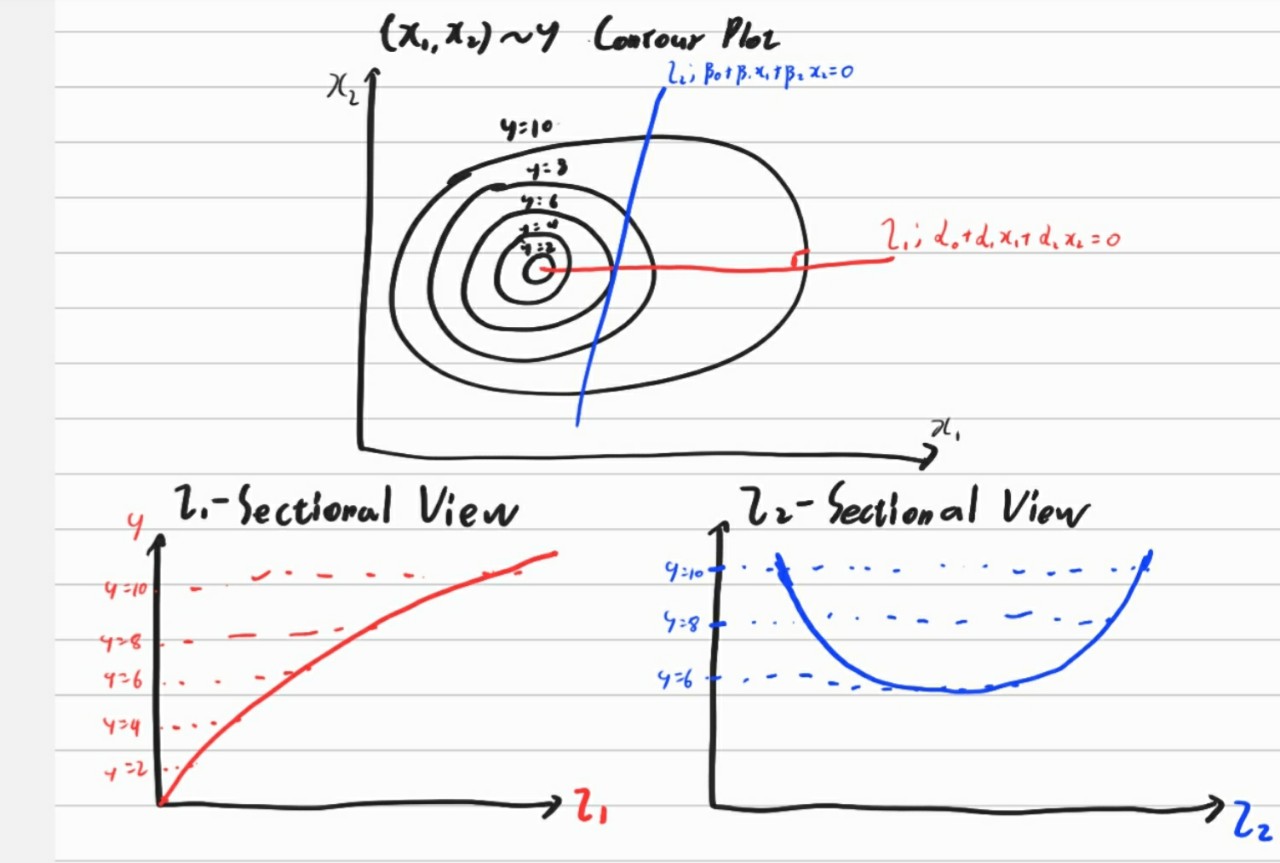
In the point of view of linear dimension reduction, l2 cannot give linear information of y. That is, correlation between l2 and y would be near to zero. On the other hand, l1 can give strong linear information of y.
CR subspace
Let $(\tilde X , \tilde Y)$ be an independent copy of $(X,Y)$. That is, suppose Y and X have the following data generating process ; $Y\mid X \sim F_{Y \mid X}(Y) $ and $X \sim F_X(x)$. And generate another independent $(\tilde X ,\tilde Y)$ using this data generating process. In practice, we can just take samples from real data. It is the same with generating from empirical distribution.
$Z,\tilde Z$ be standardized versions of $X,\tilde X$. i.e. $Z = \Sigma^{-1/2}(X-E(X)) , $and $\tilde Z = \Sigma^{-1/2}(\tilde X - E(X))$.
With above setting, CR needs following Matrix
$A(\epsilon) = E((Z-\tilde Z)(Z-\tilde Z)^t \mid \mid Y- \tilde Y\mid < \epsilon)$
and we can get theorems like before.
Theorem
If $LCM(\beta)$ and $CCV(\beta)$ are satisfied, where $\beta$ is a basis matrix of $S_{Y \mid Z}$, then $span (2 I_p - A(\epsilon)) \subset S_{Y \mid Z}$
pf)
By definition,
$A(\epsilon) = E(ZZ^t \mid \mid Y- \tilde Y \mid <\epsilon)-E(Z\tilde Z^t \mid \mid Y- \tilde Y \mid <\epsilon)-E(\tilde ZZ^t \mid \mid Y- \tilde Y \mid <\epsilon)+E(\tilde Z \tilde Z^t \mid \mid Y- \tilde Y \mid <\epsilon)$
Because $(Z,Y,\tilde Y)$ has same distribution with $(\tilde Z , Y, \tilde Y)$, $(Z \mid (Y , \tilde Y))$ and $(\tilde Z \mid (Y , \tilde Y))$ have same distribution too. This results in the following equations.
$E(Z \tilde Z^t \mid \mid Y - \tilde Y \mid < \epsilon) = E(\tilde Z Z^t \mid \mid Y - \tilde Y \mid < \epsilon)$
$E(Z Z^t \mid \mid Y - \tilde Y \mid < \epsilon) = E(\tilde Z \tilde Z^t \mid \mid Y - \tilde Y \mid < \epsilon)$
Notice that two equations are in different situations because the above equation is the product of two independent variables and below one is the second moment of a random variable. It is same situation with $E(Y)E(Z)$ is different with $ E(YZ)$
Anyway, by using above equations, we can get $A(\epsilon) = 2E(ZZ^t \mid \mid Y-\tilde Y \mid <\epsilon) - 2E(Z \tilde Z^t \mid \mid Y- \tilde Y \mid <\epsilon)$
Additionally, $(Z,Y) \perp (\tilde Z , \tilde Y) \Rightarrow Z \perp \tilde Z \mid (Y, \tilde Y)$. Therefore, above equation becomes $A(\epsilon) = 2E(ZZ^t \mid \mid Y-\tilde Y \mid <\epsilon) - 2E(Z \mid \mid Y- \tilde Y \mid <\epsilon)(Z^t \mid \mid Y- \tilde Y \mid <\epsilon)$
Now, let’s figure out how this term can be changed with LCM and CCV assumptions.
Remark if LCM assumption holds, then $E(X \mid Y) = P_{\beta}^t(\Sigma) E(X \mid Y)$ and if CCV assumption holds, then $Var(X \mid Y) = \Sigma Q_{\beta}(\Sigma) + P_{\beta}^t(\Sigma)Var(Z \mid Y) P_{\beta}(\Sigma)$ where $Q_{\beta}(\Sigma) = I-P_{\beta}(\Sigma)$
In our case, we already standardize them, so $\Sigma = I$.
$E(Z \mid \mid Y- \tilde Y \mid <\epsilon) = E(E(Z \mid Y) \mid \mid Y - \tilde Y \mid < \epsilon) = P_{\beta}^t E(E(Z\mid Y) \mid \mid Y- \tilde Y \mid <\epsilon)$
$=P_{\beta}^tE(Z\mid \mid Y- \tilde Y \mid <\epsilon)$
$E(ZZ^t \mid Y) = Var(Z \mid Y) +E(Z \mid Y)E(Z^t \mid Y)$
$= Q_{\beta} +P_{\beta}^tVar(Z \mid Y) P_{\beta} + P_\beta^t E(Z \mid Y)E(Z^t \mid Y)P_{\beta}$
$= Q_{\beta}+ P_{\beta}^tE(Z Z^t \mid Y) P_{\beta}$
$E(ZZ^t\mid \mid Y- \tilde Y \mid <\epsilon) = E(E(ZZ^t \mid Y) \mid \mid Y- \tilde Y \mid <\epsilon)$
$=E(Q_{\beta} + P_{\beta}^tE(Z Z^t \mid Y) P_{\beta} \mid \mid Y - \tilde Y \mid <\epsilon)$
$= Q_{\beta} + P_{\beta}^t E(ZZ^t \mid \mid Y - \tilde Y\mid<\epsilon)P_{\beta}$
To substitute every term in $A(\epsilon)$ with above results, then we can get $A(\epsilon) = 2Q_{\beta} + P_{\beta} A(\epsilon)P_{\beta}$
$A(\epsilon) = 2I - 2P_{\beta} + P_{\beta} A(\epsilon) P_{\beta}$
$\Rightarrow A(\epsilon) - 2I = P_{\beta}(A_{\epsilon}-2I)P_{\beta} \in span(P_{\beta}) = S_{Y \mid X}$ $\square$
And again, it can be denoted as follows.
$span(2I - A(\epsilon)) = span((2I-A(\epsilon))^2) =:span(\Lambda_{CR}) \subset S_{Y \mid X} $
Second term can be done with the lemma used in SAVE
Lemma. If U is a random matrix whose entries are square integrable, and S is a subspace of $R^p$, then $span(U) \subset S \quad a.s.P \iff span(E(U U^t)) \subset S$
Notice that purpose in proof of SIR,SAVE,CR is to show that left side of equation does not contains $P_{\beta}$ and right side of equation have to start with $P_{\beta}$
This fact implies that left side have to be calculated in the situation that $P_{\beta}$ is unknown and right side become element of column space of $P_{\beta}$ i.e. SDR subspace. Therefore, in the whole procedure, we can derive a certain basis without $P_{\beta}$ but it goes to $P_{\beta}$.
Notice too that the procedure has some part of imperfection that v cannot give confidence that our term can give the entire SDR space.
In detail, SDR subspace is $span(P_{\beta}) = {P_{\beta} v : v \mbox{ is any vector in } R^n}$ but our result is $span(\Lambda) = {P_{\beta} v: v \mbox{ have to be in certain form}}$.
Therefore, we cannot say that $span(\Lambda) = span(P_{\beta})$ but we can only say $span(\Lambda) \subset span(P_{\beta})$
Exhaustiveness of Contour Regression
For the above reason, if we can say $span(\Lambda) \supset span(P_{\beta})$, then we can conclude $span(\Lambda) = span(P_{\beta})$. Like SAVE, there is a condition which can make it possible.
Theorem
Suppose $LCM(\beta)$ and $CCV(\beta)$ are held. Suppose $(\tilde Z , \tilde Y)$ is an independent copy of $(Z,Y)$ and $\epsilon$ >0 . If , for any $v \in S_{Y \mid Z},$ we have $E([v^t(Z- \tilde Z)]^2 \mid \mid Y - \tilde Y \mid <\epsilon) < E([v^t (Z- \tilde Z)]^2)$, then $span(\Lambda_{CR}) = S_{Y \mid Z}$
Above condition seems generally applicable. $[v^t (Z- \tilde Z)]^2$ means variance of Z and it is reasonable to think that if z and y have some connection, then the variance of Z which has small Z would be small too.
2. Directional Regression
Contour regression can show quite good performance but it also has a big computing cost. Therefore, advanced algorithms aim to make computation costs smaller. The result of this move is a directional regression algorithm.
Remark that contour regression is based on the matrix $A(\epsilon) = E((Z-\tilde Z)(Z-\tilde Z)^t \mid \mid Y- \tilde Y\mid < \epsilon)$. Directional regression is based on a much simpler version of it $E((Z-\tilde Z)(Z-\tilde Z)^t \mid Y,Y)$.
To calculate $A(\epsilon) = E((Z-\tilde Z)(Z-\tilde Z)^t \mid \mid Y- \tilde Y\mid < \epsilon)$, computer have to discern the case that $\mid Y-\tilde Y \mid$ is smaller than $\epsilon$. That is similar to selecting a case.
Directional regression is similar to reorganizing in this sense. Let’s figure it out.
Theorem
If $LCM(\beta)$ and $CCV(\beta)$ are satisfied, where $\beta$ is a basis matrix of $S_{Y \mid Z}$, then $span (2 I_p - E((Z-\tilde Z)(Z-\tilde Z)^t \mid Y,Y)) \subset S_{Y \mid Z}$
It seems obvious when remark the SAVE subspace which states that $span(2I_p - Var(Z \mid Y)) \sub S_{Y \mid Z}$ because $Var(Z\mid Y)$ is almost same one with $E((Z-\tilde Z)(Z-\tilde Z)^t \mid Y, \tilde Y)$. Anyway, let’s prove it.
Pf)
Let $A(Y ,\tilde Y) = E((Z-\tilde Z)(Z-\tilde Z)^t \mid Y, \tilde Y)$.
Then $A(Y,\tilde Y) = E(ZZ^t\mid Y, \tilde Y) -E(Z \mid Y, \tilde Y) E(\tilde Z^t \mid Y, \tilde Y)-E(\tilde Z \mid Y, \tilde Y) E( Z^t \mid Y, \tilde Y) +E(\tilde Z \tilde Z^t \mid Y, \tilde Y)$ like CR and this also can be rewritten as $A(Y,\tilde Y) = 2 Q_\beta +P_\beta A(Y, \tilde Y) P_\beta$
Therefore, we can get $A(Y, \tilde Y) - 2I = P_\beta A(Y,\tilde Y) -2 I)P_\beta$ which is the desired result. $\square$
To find the basis of $(2I-A(Y,\tilde Y))$, we have to find the eigenvalue of the square term. Therefore, we make main matrix as $\Lambda_{dr} = (2I-A(Y , \tilde Y))^2$
And like SAVE, we can change $\Lambda _{dr}$ to the term without using $\tilde Z, \tilde Y$
$\Lambda_{dr} = 2E(E(ZZ^t \mid Y))^2 + 2E(E(Z \mid Y) E(Z^t \mid Y))^2+2E(E(Z^t \mid Y)E(Z\mid Y))E(E(Z\mid Y) E(Z^t \mid Y)) -2I_p$
The detail derivation could be done with tedious procedure, so let’s skip it.
Anyway, we can estimate DR subspace using $\Lambda_{dr}$. In this case, like SIR and SAVE, we have to estimate $E(Z \mid Y)$ and $E(ZZ^t \mid Y)$ using a slice. Actual algorithm is below.
Standardize $X_1, X_2, … , X_n$ to $Z_1, Z_2,…Z_n$
Make partition of Y with {$J_i ; i=1,2,…h$} and compute $M_{1i}=E_n(Z \mid Y \in J_i), M_{2i}=E_n(ZZ^t \mid Y \in J_i)$
Compute $\Lambda_1 = h^{-1}\sum_{i=1}^h P_n(Y\in J_i)M^2{2i}$ ; $P_n(Y \in J_i) = E_n(I(Y \in J_i))$ and $\Lambda_2 = h^{-1}\sum{i=1}^h P_n(Y\in J_i)(M_{1i}M_{1i}^t)^2$ and $\Lambda_3 = h^{-1}[\sum_{i=1}^h P_n(Y\in J_i)(M_{1i}^tM_{1i})^2][h^{-1}\sum_{i=1}^h P_n(Y\in J_i)(M_{1i}M_{1i}^t)^2]$
[Notice that $E_n(X) = n^{-1}\sum_{i=1}^n (X_i)$ i.e. sample mean]
And make matrix $\Lambda_{dr} = 2\Lambda_1 +2 \Lambda_2 +2 \Lambda_3 -2 I_p$
By solving the eigenvalue problem, we can get the desired result.
Like before, directional regression has the exhaustive condition that $E((v^t (Z-\tilde Z))^2 \mid Y ,\tilde Y)$ is non-degenerate.
Debnath, L.& Mikusinski, P. (2005). Introduction to Hilbert Space.London,UK.:Elsevier Academic Press
Li, B. (2018). Sufficient Dimension Reduction. Boca Raton,FL:CRC Press.