Non-linear Dimension Reduction - 2. Coordinate Representation and KPCA

1. Coordinate Representation on Hilbert space

어떠한 Hilbert space H에 대해서 H 내부의 모든 원소가 다른 원소 집합들의 선형결합으로 표현될 수 있다면 그 다른 원소 집합을 일컬어 Complete Basis라고 한다.

즉 어떤 원소 $x \in H$에 대해 $x = \sum_{i=1}^{\infty} x_i e_i$로 표현이 될 시 $\{e_i\}$는 complete basis라고 말할 수 있다. 이때 $e_i$마다 곱해져 있는 스칼라 값 $x_i$를 coordinate(좌표)라고 한다.

Complete basis는 힐버트 공간의 차원이 유한할 때는 반드시 존재하며, 무한할 지라도 우리가 관심있는 대부분의 공간은 이러한 Complete basis가 존재한다.

일반적으로는 선형독립인 basis를 설정하여 각 원소마다 유니크한 좌표를 뽑아내지만, 굳이 베이시스가 선형독립일 필요는 없다.

따라서 우리는 좀 더 느슨하게 정의된 베이시스를 이용하여, 함수조차도 좌표를 이용해서 표현할 수 있다.

구체적으로 다음과 같이 정의하자. $\def\coor#1#2{\left[ #1 \right]_{\mathfrak{#2}}}$ $\def\inn#1{\left<#1\right>}$

Coordinate representation of Elements

For any $f \in H$ with spanning system $\{b_1,b_2,...b_m\}$, there is coordinates $(c_1,c_2,...,c_m)$ such that $f = c_1b_1+c_2b_2+...+c_m b_m$.

Let’s denote basis as $b_{1:m}$ and coordinates $\coor{f}{B}=(c_1,c_2,...,c_m)^t$, then $f = \coor{f}{B}^t b_{1:m}$.

베이시스를 유한개로 한정지은 것과 베이시스간 직교성은 없다는 것에 유의하자.

이 경우, 베이시스를 규정해 놓으면 $f$를 대표해서 $\coor{f}{B}$를 대신 사용할 수 있다.

이제 이를 RKHS에 적용해서 발전시켜보자. RKHS에서는 내적이 다음과 같이 정의된다.

For $f = \sum f_i k(\cdot,s_i)$, $g = \sum g_i k(\cdot,s_i)$, the inner product $\inn{f,g}_{H} = \sum_i \sum_j f_i g_j k(s_i,s_j)$

여기서 베이시스 $b_i = k(\cdot, s_i)$이며, $\inn{b_i,b_j} = k(s_i,s_j)$임을 유의하자. 이 내적을 위의 coordinates representation을 이용해서 표현하면 다음과 같다.

Coordinate representation of Inner Product
\[\inn{f,g}_{H} = \sum_i \sum_j (\coor{f}{B})_i (\coor{g}{B})_j k(s_i,s_j) =: \coor{f}{B}^t G_{\mathfrak{B}}\coor{g}{B}\]
where $G_{\mathfrak{B}} = \{k(s_i,s_j)\}_{ij}$ and called as Gram Matrix

Gram Matrix는 basis가 되는 모든 커널들을 내적해서 표현한 행렬의 형태이다.

다음으로 힐버트 공간에서 정의되는 Linear Operator도 살펴보자.

Let $A: H_1 \rightarrow H_2$ be a linear operator where $H_1 = span(b_{1}^{(1)} ,b_{2}^{(1)} ,...,b_{n}^{(1)})$ and $H_2 = span(b_{1}^{(2)} ,b_{2}^{(2)} ,...,b_{m}^{(2)})$ , then

\[Af = A\sum_i (\coor{f}{B})_i b_i^{(1)}\]

$= \sum_i (\coor{f}{B})_i A b_i^{(1)} = \sum_i (\coor{f}{B})_i \sum_j (\coor{A b_i^{(1)}}{B2})_j b_j^{(2)}$

$= \sum_j [\sum_i (\coor{f}{B})_i (\coor{A b_i^{(1)}}{B2})_j] b_j^{(2)}$

여기서 가온데 항 $[\sum_i (\coor{f}{B})_i (\coor{A b_i^{(1)}}{B2})_j]$는 스칼라 값이다. 따라서 위는 아래와 같이 표기할 수 있다.

$=: \sum_j (\coor{A_f}{B2})_j b_j^{(2)}$

$=: \coor{Af}{B2} b^{(2)}$

여기서 $[\sum_i (\coor{f}{B1})_i (\coor{A b_i^{(1)}}{B2})_j]$ 항은 다시 행렬의 형태로 표현 될 수 있다. 즉 다음과 같다.

\[\coor{Af}{B2} = \left[ \begin{array}{c} [\sum_i (\coor{f}{B1})_i (\coor{A b_i^{(1)}}{B2})_1] \\\ [\sum_i (\coor{f}{B1})_i (\coor{A b_i^{(1)}}{B2})_2] \\\ \vdots \\\ [\sum_i (\coor{f}{B1})_i (\coor{A b_i^{(1)}}{B2})_n] \end{array} \right]\]

$= \left[ \begin{array}{cccc} (\coor{A b_i^{(1)}}{B2})_1 &(\coor{A b_i^{(1)}}{B2})_1 & \cdots &(\coor{A b_i^{(1)}}{B2})_1 \\\ (\coor{A b_i^{(1)}}{B2})_2 &(\coor{A b_i^{(1)}}{B2})_2 & \cdots &(\coor{A b_i^{(1)}}{B2})_2 \\\ \vdots & \vdots & \ddots & \vdots \\\ (\coor{A b_i^{(1)}}{B2})_n &(\coor{A b_i^{(1)}}{B2})_n & \cdots &(\coor{A b_i^{(1)}}{B2})_n \end{array} \right]\left[ \begin{array}{c} (\coor{f}{B1})_1 \\\ (\coor{f}{B1})_2\\\ \vdots \\\ (\coor{f}{B1})_m\end{array} \right]$

$=: (_{\mathfrak{B2}}\coor{A}{B1}) \coor{f}{B1}$

즉 오퍼레이터 A는 A를 두 베이시스를 통해 평가한 원소가 들어가게 된다. $\{A_{ij}\} =(\coor{A b_i^{(1)}}{B2})_j$

추가적으로 만약 베이시스들이 orthonormal basis라면 $\{A_{ij}\} = \inn{Ab_i^{(1)},b_j^{(2)}}$가 된다.

이를 정의내리면 다음과 같다.

Coordinate representation of Linear Operator
\[Af = (_{\mathfrak{B2}}\coor{A}{B1}) \coor{f}{B1} b^{(1)}\]
where $G_{\mathfrak{B}} = \{\inn{s_i,s_j}\}_{ij}$ and called as Gram Matrix

일반적으로 RKHS에서의 오퍼레이터는 대부분 tensor product의 형태로 구성된다. 만약 오퍼레이터가 tensor product일시 다음과 같이 더 직관적인 형태로 변한다.

\[\coor{(g\otimes f) b_i^{(1)}}{B2} = \coor{g}{B2} \inn{f , b_i ^{(1)}}_{H1} = \coor{g}{B2} \coor{f}{B1}^t G_{\mathfrak{B1}} \coor{b_i^{(1)}}{B1}\]

여기서 $\coor{b_i^{(1)}}{B1}$은 basis $b_i$의 coordinate를 의미하므로 i번째 값만 1이고 나머지는 모두 0이다. 따라서 $\coor{b_i^{(1)}}{B1} = e_i$이다.

따라서 $\left\{\coor{(g\otimes f) b_i^{(1)}}{B2}\right\}_i = \coor{g}{B2} \coor{f}{B1}^t G_{\mathfrak{B1}} (e_1,e_2,...e_m) = \coor{g}{B2} \coor{f}{B1}^t G_{\mathfrak{B1}}$이다.

Coordinate representation of Linear Operator with tensor product
\[(_{\mathfrak{B2}}\coor{(g\otimes f) }{B1}) = \coor{g}{B2} \coor{f}{B1}^t G_{\mathfrak{B1}}\]
where $G_{\mathfrak{B}} = \{\inn{s_i,s_j}\}_{ij}$ and called as Gram Matrix

결과적으로 내적을 정의함으로써 힐버트 공간에 존재하는 삼대 요소인 원소, 내적, 작용소를 모두 기존의 선형대수학에서 사용하는 벡터-행렬 노테이션으로 완벽하게 표현할 수 있다. 이는 곧 함수와 오퍼레이터가 인풋이고 유클리드 공간의 벡터나 행렬이 아웃풋인 맵핑을 얻은 것이다. 이를 다음과 같이 정리하자.

Coordinate Mapping
\[\coor{\cdot}{B1} : H_1 \rightarrow \mathbb{R}^{m_1} , \coor{f}{B1}\] \[(_{\mathfrak{B2}}\coor{\cdot}{B1}) : B(H_1,H_2) \rightarrow \mathbb{R}^{m_2 \times m_1} , (_{\mathfrak{B2}}\coor{A}{B1})\]

이 맵핑은 다음과 같은 성질을 가진다.

Evaluation: $\coor{Th}{B2} = (_{\mathfrak{B1}} \coor{T}{B1})\coor{h}{B1}$

Linearity: $\coor{\alpha_1 f_1 + \alpha_2 f_2}{B1} = \alpha_1\coor{ f_1}{B1} + \alpha_2\coor{f_2}{B1}$
\[(_{\mathfrak{B2}}\coor{\alpha_1 T_1 + \alpha_2 T_2}{B1}) = \alpha_1(_{\mathfrak{B2}}\coor{ T_1}{B1}) + \alpha_2(_{\mathfrak{B2}}\coor{T_2}{B1})\]

Composition: $(_{\mathfrak{B3}} \coor{T_2T_1}{B1}) = (_{\mathfrak{B3}} \coor{T_2}{B2})(_{\mathfrak{B2}} \coor{T_1}{B1})$

Inner Product $\inn{f,g}_{H} = [f]_{\mathfrak{B}}^t G_{\mathfrak{B}}[g]_{\mathfrak{B}}$

Tensor Product $(_{\mathfrak{B2}}\coor{(g\otimes f) }{B1}) = \coor{g}{B2} \coor{f}{B1}^t G_{\mathfrak{B1}}$

2. Coordinate Representation on Hilbert space

앞선 포스팅에서는 $ker(\Sigma_{xx})$를 $\{0\}$으로 가정하고 $\bar{ran}(\Sigma_{xx}) = H_x$를 만들었다. 이 말은 $\bar{ran}(\hat{\Sigma}_{xx}) = span(k(\cdot , X_i)- E_n(k(\cdot,X):i=1,2,...n)$ 이므로 $H_x$의 베이시스로 $\{k(\cdot , X_i)- E_n(k(\cdot , X))\} = \{b_i^{(X)}\}$를 사용할 수 있음을 의미한다.

이에 대해서 covariance operator $\Sigma_{xx},\Sigma_{xy},\Sigma_{yy}$의 coordinate mapping을 구해보자.

\[\hat{\Sigma}_{xx} = E_n([k(\cdot , X_i)-E_n(k(\cdot , X))] \otimes [k(\cdot , X_i)-E_n(k(\cdot , X))]) = \frac{1}{n} \sum_{i=1}^{m} b_i^{(X)} \otimes b_i^{(X)}\]

이에 대해서 다음과 같은 전개가 성립한다.

\[\coor{\hat{\Sigma}_{xx} b_i^{(X)}}{Bx} = n^{-1}\coor{\sum_{i=1}^m (b_k^{(X)}\otimes b_k^{(X)}) b_i^{(X)}}{Bx}\]

$= n^{-1}\sum_{i=1}^m \coor{(b_k^{(X)}\otimes b_k^{(X)}) b_i^{(X)}}{Bx}$

$= n^{-1}\sum_{i=1}^m \coor{b_k^{(X)}}{Bx}\coor{b_k^{(X)}}{Bx}^t G_{\mathfrak{Bx}} \coor{ b_i^{(X)}}{Bx}$

$= n^{-1} \sum_{i=1}^{m} e_k e_k^t G_{\mathfrak{Bx}} e_i$

$= n^{-1} G_{\mathfrak{Bx}} e_i$

따라서 $(_{\mathfrak{Bx}}\coor{\hat{\Sigma}_{xx}}{Bx}) = n^{-1} G_{\mathfrak{Bx}}$이다.

이때 그람 행렬은 다음과 같이 분해 된다.

\[G_{\mathfrak{Bx}} = (\inn{b_i^{(X)} , b_j^{(X)}})_{ij} = \inn{[k(\cdot , X_i)-n^{-1} \sum (k(\cdot , X))],[k(\cdot , X_i)-n^{-1} \sum (k(\cdot , X))]}\]

$= (k(X_i,X_j) - n^{-1}\sum_l k(X_i,X_l)- n^{-1}\sum_k k(X_i,X_k) + n^{-2} \sum \sum k(X_l,X_k))$

이는 커널매트릭스 $K_x = \{k(X_i,X_j)\}_{ij}$의 $Q = I_n - n^{-1} 1_n1_n^t$에 대한 프로젝션이다. 따라서 $G_{\mathfrak{Bx}} = QK_xQ$가 성립한다.

마찬가지로 $(_{\mathfrak{Bx}}\coor{\hat{\Sigma}_{yy}}{Bx}) = n^{-1} G_{\mathfrak{By}}$가 성립한다.

다음으로 Covariance Operator $\hat{\Sigma}_{yx} = n^{-1}\sum b_i^{(Y)} \otimes b_i^{(X)}$에 대해서 분석해보자.

\[[\hat{\Sigma}_{yx} b_i^{(x)}]_{\mathfrak{By}} = [(n^{-1}\sum b_i^{(Y)} \otimes b_i^{(X)})b_j^{(X)}]_{\mathfrak{By}}\]

$= n^{-1} \sum [b_i^{(y)}]_{\mathfrak{By}} [b_i^{(x)}]_{\mathfrak{Bx}}^t G_{\mathfrak{Bx}}[b_j^{(x)}]_{\mathfrak{Bx}}$

$=n^{-1}\sum e_i e_i^t G_{\mathfrak{Bx}} e_j = n^{-1} G_{\mathfrak{Bx}}e_j$

따라서 $(_{\mathfrak{By}}\coor{\hat{\Sigma}_{yx}}{Bx}) = n^{-1} G_{\mathfrak{Bx}}$가 성립한다.

결론적으로 다음과 같이 정리할 수 있다.

\[(_{\mathfrak{Bx}}\coor{\hat{\Sigma}_{xx}}{Bx}) = n^{-1} G_{\mathfrak{Bx}}\] \[(_{\mathfrak{Bx}}\coor{\hat{\Sigma}_{yy}}{Bx}) = n^{-1} G_{\mathfrak{By}}\] \[(_{\mathfrak{By}}\coor{\hat{\Sigma}_{yx}}{Bx}) = n^{-1} G_{\mathfrak{Bx}}\] \[(_{\mathfrak{Bx}}\coor{\hat{\Sigma}_{xy}}{By}) = n^{-1} G_{\mathfrak{By}}\]

3. Kernel PCA

이 RKHS를 이용하면 PCA를 non-linear에서 진행할 수 있다.

일반적인 PCA는 다음과 같다.

\[\max Var(\delta^t X)\] \[\mbox{subject to } \delta^t \delta =1\]

이는 X의 변수들을 선형결합해서 새로 변수를 만드는데, 그 기준을 variance가 최대치가 되게끔 만들어내는 알고리즘이다.

이를 라그랑주 방법론을 이용하면 다음과 같이 풀린다.

\[\frac{d}{d \delta} (\delta^t \Sigma_{xx} \delta -\lambda (\delta^t \delta -1) = 2 \Sigma \delta -2\lambda \delta =0\]

이를 풀면 $\Sigma \delta = \lambda \delta$가 되며, 이는 eigen value의 정의와 일치한다.

그러나 이 PCA는 새로운 변수를 선형결합으로만 찾는다는 한계점이 있다. 따라서 이러한 한계점을 풀고 일반화 하면 문제는 다음과 같이 바뀐다.

\[\max Var(f(X))\] \[\mbox{subject to } \parallel f \parallel_{H}=1\]

이에 대해서 RKHS를 이용하면 $Var(f(X)) = \inn{f, \Sigma_{xx} f}_{H}$가 성립하는 것을 알 수 있다. 따라서 문제는 다음과 같이 바뀐다.

\[Var(f(X)) = \inn{f , \Sigma_{xx} f }_{H} = \coor{f}{Bx}^t G_{\mathfrak{Bx}}(_{\mathfrak{Bx}}\coor{\hat{\Sigma}_{xx}}{Bx})\coor{f}{Bx} = n^{-1}\coor{f}{Bx}^t G_{\mathfrak{Bx}}^2 \coor{f}{Bx}\] \[\parallel f \parallel_H = \inn{f,f}_{H} = \coor{f}{Bx}^t G_{\mathfrak{Bx}}\coor{f}{Bx}\]

따라서 KPCA 문제는 다음과 같이 변형된다.

\[\max \coor{f}{Bx}^t G_{\mathfrak{Bx}}^2 \coor{f}{Bx}\] \[\mbox{subject to } \coor{f}{Bx}^t G_{\mathfrak{Bx}} \coor{f}{Bx} = 1\]

이는 일반적인 $GEV( G_{\mathfrak{Bx}}^2, G_{\mathfrak{Bx}})$로 단순화시켜서 풀 수 있다.

좀 더 구체적으로 보기 위해서 구현까지 진행해보자.

Algorithm. Kernel PCA

Standardized $X_i$
Choose Kernel Function and compute kernel matrix $K_X$
Compute Gram Matrix $G_X$ and decompose it.

사용된 코드는 다음과 같다.

stand(data):return(np.apply_along_axis(np.var, 0, X)**(-0.5)*(X - np.apply_along_axis(sum, 0, X)))
def Gram(data) : 
    n = X.shape[0];p = X.shape[1] 
    U = np.matmul(X,X.T)
    M = np.outer(np.diag(U),np.ones(shape=(n,1)))
    J = np.outer(np.ones(shape=(n,1)),np.ones(shape=(n,1)))
    Q = np.identity(n)-J/n
    K = M+M.T-2*U
    sigma = n*(n-1)/(np.sum(np.sqrt(K))-np.trace(np.sqrt(K)))/2
    return(np.matmul(Q,np.exp(-(M+M.T-2*U)/sigma/sigma),Q))
def matpower(mat,power,thre):
    eig = np.linalg.eig(mat)
    val = np.diag([np.real(i**power) if i >thre else 0 for i in eig[0]])
    vec = np.real(eig[1])
    return(np.matmul(np.matmul(vec,val),vec.T))

위는 matrix power를 효율적으로 해주는 함수와 표준화를 해주는 함수 그리고 그람행렬을 구해주는 함수로 구성되어 있다.

def KPCA(data,thre = 10**(-8)):
    #1. 그람 행렬 계산
    G = Gram(data)
    #2. 그람 행렬 분해
    eig = np.linalg.eig(G)
    V = np.real(eig[1])
    #3. 제약 보정
    U = np.matmul(matpower(G,-0.5,10**(-8)),V)
    #4. PC축 계산
    return(np.matmul(G,U))

본격적인 KPCA 코드는 위와 같다. 1. Gram 행렬을 만들어 준 뒤 2.이를 분해해주고 3.$\coor{f}{Bx}^t G_{\mathfrak{Bx}} \coor{f}{Bx} = 1$에 대한 보정을 진행한 결과이다.

4번째 과정은 다음과 같은 논리로서 만들어진다.

\[u_i = \coor{\underset{f}{\arg \max} \quad var(f(X))}{Bx} = \coor{f_i}{Bx}\]

PC components

\[z_i = \left[ \begin{array}{c} f_i(x_1) \\\ f_i(x_2) \\\ \vdots \\\ f_i(x_n) \end{array}\right] = \left[ \begin{array}{c} \inn{f_i,K(\cdot , x_1)} \\\ \inn{f_i,K(\cdot , x_2)} \\\ \vdots \\\ \inn{f_i,K(\cdot , x_n)} \end{array}\right] = \left[ \begin{array}{c} \coor{K(\cdot , x_1)}{Bx}^t G_x \coor{f_i}{Bx} \\\ \coor{K(\cdot , x_2)}{Bx}^t G_x \coor{f_i}{Bx} \\\ \vdots \\\ \coor{K(\cdot , x_n)}{Bx}^t G_x \coor{f_i}{Bx} \end{array}\right]= \left[ \begin{array}{c} \coor{K(\cdot , x_1)}{Bx}^t G_x u_i \\\ \coor{K(\cdot , x_2)}{Bx}^t G_x u_i \\\ \vdots \\\ \coor{K(\cdot , x_n)}{Bx}^t G_x u_i \end{array}\right]\]

여기서 $k(\cdot , x_i)$는 베이시스 그 자체 이므로 $\coor{k(\cdot , x_i)}{Bx} = e_i$이다. 따라서 위의 식은 다음과 같이 바뀐다.

\[z_i = IG_{x}u_i = G_x u_i\]

i 행렬을 모두 복원 한다면 GU가 모든 정보량을 보존한 행렬이 되며 가장 앞에 있는 열이 메인 KPCA열이 된다.

이를 이용하면 다음과 같은 자료를 만들 수 있다.

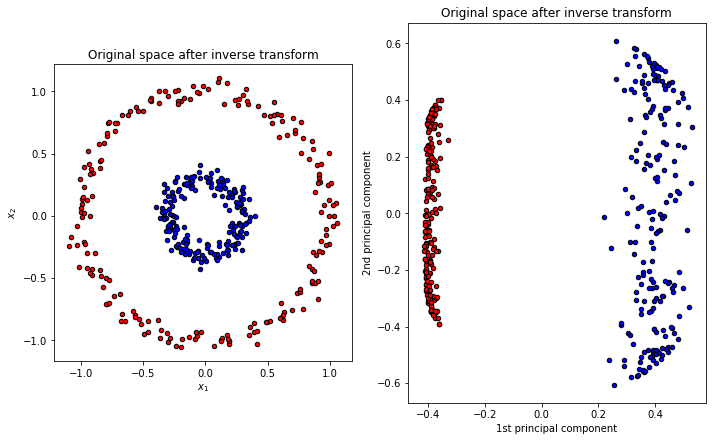
지금까지 RKHS의 유클리드 공간에서의 표기법 및 그를 이용한 KPCA까지 구현을 진행해보았다. 다음 포스팅 에서는 Sliced Inverse Regression을 Nonlinear을 이용해서 진행해보자.

Debnath, L.& Mikusinski, P. (2005). Introduction to Hilbert Space.London,UK.:Elsevire Academic Press
Li, B. (2018). Sufficient Dimension Reduction. Boca Raton,FL:CRC Press.

Twitter Facebook LinkedIn

[Non-linear Dimension Reduction] Part 2. Coordinate Representation and KPCA

Dimensionality Reduction

Non-linear Dimension Reduction - 2. Coordinate Representation and KPCA

1. Coordinate Representation on Hilbert space

2. Coordinate Representation on Hilbert space

3. Kernel PCA

You May Also Enjoy

[Paper Review] Dimensionality Reduction as Probabilistic Inference

[Paper Review] Dimensionality Reduction as Probabilistic Inference

계속 쓰는 시

6월의 시