개요

이번 베이즈 과제는 GMM을 따르는 데이터에 대해서 각 자료마다 속해있는 군집에 대한 지표인 Latent Variable $z_i$를 Gibbs Sampler와 EM Algorithm을 이용하여 찾아내는 것이다.

우선 자료의 모양을 보면 다음과 같다.

data = read.csv("data_mixture.csv")
data %>%
 ggplot(aes(x))+geom_histogram()

겉으로 보았을 때 4개의 군집이 섞여있는 GMM 꼴로 보인다. 따라서 찾아줄 잠재변수의 개수를 4개로 한정지을 수 있다.

본격적으로 찾아주기에 앞서 분포들을 가정하자

데이터 분포 가정

$Y_i \sim \sum^{4}_{k=1}\pi_kN(y_i;u_k,\tau_k)$

$Prior 분포 가정$

$(\pi_1,\pi_2,\pi_3,\pi_4) \sim Diri(a)$ $\mu_k \sim N(\gamma,\kappa) , \tau_k \sim IG(a,b)$ $z_i \sim Multi(\pi_1,\pi_2,\pi_3,\pi_4)$

Gibbs Sampler로 Latent Variable 찾아내기

우선 prior 분포의 상수부들을 설정해주자

alpha = 1

gamma = 5
kappa = 1

a = 1
b = 1

그다음으로 각 분포의 초기값들을 설정해주자

iter=10000

K = 4
pi_temp = c(0.25,0.25,0.25,0.25)
mu_temp = c(1,5,7,15)
tau_temp = c(1,1,4,7)

z_temp = c()
for (i in c(1:dim(data)[1])){
  if(data[i,2] < 3){zi = 1}
  else if(data[i,2]<7){zi = 2}
  else if(data[i,2]<12){zi = 3}
  else{zi=4}
  z_temp = append(z_temp,zi)
}

z_temp <- as.factor(z_temp)

pi_post=pi_temp
mu_post=mu_temp
tau_post=tau_temp
z_post=z_temp

이제 full-conditional distribution을 찾아주자

Gibbs Sampler를 위해서는 Full Conditional Distribution을 찾아줄 필요가 있다. 따라서 베이즈 룰을 이용하여 사후분포의 꼴을 찾아주면 다음과 같다.

$p(z,\pi,\mu,\tau \mid D) \propto p(D \mid z,\pi, \mu, \tau)\times p(z,\pi,\mu,\tau)$
$\ \ \ \ \ \ \ \ \ \ \ \ \ \ \ \ \ \ \ \ \ \ \ \ =p(D \mid z,\pi,\mu,\tau)\times p(z,\pi)\times p(\mu) \times p(\tau)$
$\ \ \ \ \ \ \ \ \ \ \ \ \ \ \ \ \ \ \ \ \ \ \ \ =p(D \mid z,\pi,\mu,\tau)\times p(z \mid \pi)\times p(\pi)\times p(\mu) \times p(\tau)$
$\ \ \ \ \ \ \ \ \ \ \ \ \ \ \ \ \ \ \ \ \ \ \ \ =\prod\prod N(y_i;\mu_k,\tau_k)^{I(z_i=k)}\prod Multi(z_i; \pi) \times Diri(\pi;\alpha)\prod N(\mu_k;0, \kappa ) \prod IG(\tau_k;a,b)$

1. $\mu,\tau$의 FCD 체크하기

위의 분포를 그대로 보면 무진장 복잡해지지만 k끼리는 서로 독립이라는 점을 염두에 둔다면 포착대상 이외는 모두 상수로써 사라진다는 것을 알 수 있다.

또한 $z_i=\theta$인 경우만 염두에 둔다면 $z_i=\theta$가 아닌 데이터 y들은 $\mu_\theta,\tau_\theta$를 결정하는것에 영향을 미치지 않는다. 따라서 아래와 같이 써줄 수 있다.

$D_\theta \equiv {y_i \mid z_i = \theta}$ 로 둘시
$\propto N(D_{\theta}; \mu_{\theta}, \tau_{\theta}) \pi_{\theta} Diri( \pi, \alpha) N( \mu_{\theta};\gamma, \kappa) IG( \tau_{\theta};a,b)$

여기서 디리클레 분포 부분과 $\pi_{\theta}$는 $\mu_\theta,\tau_\theta$와 무관하므로 상수처리되므로 남은 부분은 다음과 같다.
$\propto N(D_{\theta}; \mu_{\theta}, \tau_{\theta}) N( \mu_{\theta};\gamma, \kappa) IG( \tau_{\theta};a,b)$

$\theta$가 픽스된 부분임을 감안한다면 위의 꼴은 일반적인 정규분포의 density꼴과 같으며 $\mu_{\theta},\tau_{\theta}$는 conjugate 분포의 꼴을 가지므로 공식을 그대로 사용해서 다음과 같은 fullcondition distribution을 뽑아낼 수 있다.

$p(\mu_{\theta} \mid D,z,\pi,\tau)=p(\mu_{\theta} \mid D_\theta)$
$= N(\frac{\frac{1}{\kappa}\gamma+\frac{n_h}{\sigma_h^2}\bar{y_{\theta}}}{\frac{1}{\kappa}+\frac{n_h}{\sigma_h^2}},(\frac{1}{\kappa}+\frac{n_h}{\sigma_h^2})^{-1})$

$p(\tau_{\theta} \mid D,z,\pi,\mu)=p(\tau_{\theta} \mid D_{\theta})$
$=IG(a+\frac{n_{\theta}}{2},b+\frac{\sum(y_i-\mu_{\theta})^2}{2})$

2. $\pi,z_i$의 FCD 체크하기

$\pi_k$는 $\mu_{\theta},\tau_{\theta}$와는 무관하게 정해진다. 또한 디리클레 분포는 다항 분포의 conjugate prior분포이므로 다음과 같은 posterior꼴을 가진다.
$p(\pi_k \mid D,\mu,\tau,z) = p(\pi_k \mid D) = Diri(\alpha+n_1,\alpha+n_2,…,\alpha+nk)$

마지막으로 Latent Index $z_i$는 다음과 같은 분포를 가진다. $p(z_i=k \mid D) = p(z_i \mid \pi_k) =Mul({\frac{\pi_kN(x_i;\mu_k,\tau_k)}{\sum\pi_kN(x_i;\mu_k,\tau_k)}}_{k=1}^K)$

위에서 구한 분포들을 이용하여 Gibbs Sampler 코드를 짜면 다음과 같다.

for (it in 1:iter){

## pi 샘플링
diri_index= c()
for (i in 1:K) {
  diri_index = append(diri_index,alpha + sum(z_temp==as.character(i)))
}
pi_temp <- rdirichlet(1,diri_index)

## mu 샘플링
mu_temp = c()
for (i in 1:K){
  data_mu = data[z_temp==i,2]
  n = length(data_mu)
  y_bar = mean(data_mu)
  y_sigma = tau_temp[i]
  condi_mean = (gamma/kappa+n*y_bar/y_sigma)*(1/kappa+n/y_sigma)^(-1)
  condi_var =  (1/kappa+n/y_sigma)^(-0.5)
  mu_temp = append(mu_temp,rnorm(1,condi_mean,condi_var))
}

## tau 샘플링
tau_temp = c()
for (i in 1:K){
  data_tau = data[z_temp==i,2]
  n = length(data_tau)
  dev = sum((data_tau-mu_temp[i])^2)
  condi_a = a+n/2
  condi_b = b+dev/2
  tau_current = rinvgamma(1,condi_a,condi_b)
  if (tau_current>50){tau_current = 50}
  tau_temp = append(tau_temp,tau_current)
}

# latent index 샘플링
z_temp = c()
for (i in 1:dim(data)[1]){
  
  over_density = c()
  
  for (k in 1:K){
    kprob = dnorm(data[i,2],mu_temp[k],tau_temp[k]^(0.5))*pi_temp[k]
    over_density = append(over_density,kprob)
  }
  under_density = sum(over_density)
  
  prob = over_density/under_density
  
  z_ind = sample(c(1:K),1,prob=prob)
  
  z_temp = append(z_temp,z_ind)
}


## sample 저장
pi_post = rbind(pi_post,pi_temp)
mu_post = rbind(mu_post,mu_temp)
tau_post = rbind(tau_post,tau_temp)
z_post = rbind(z_post,z_temp)
}

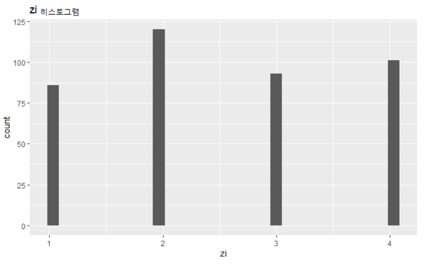
Gibbs Sampler의 결과물로 예측해낸 라벨의 분포는 다음과 같다.

p1 <- ggplot() + geom_histogram(aes(z_temp))  + ggtitle("zi 히스토그램") + xlab("zi")
p1

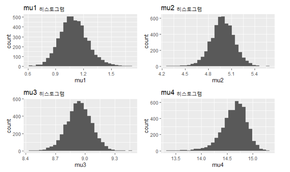
군집들의 평균에 대한 예측분포는 다음과 같다.

p2 <- ggplot() + geom_histogram(aes(mu_post[5000:10000,1]))  + ggtitle("mu1 히스토그램") + xlab("mu1")
p3 <- ggplot() + geom_histogram(aes(mu_post[5000:10000,2]))  + ggtitle("mu2 히스토그램") + xlab("mu2")
p4 <- ggplot() + geom_histogram(aes(mu_post[5000:10000,3]))  + ggtitle("mu3 히스토그램") + xlab("mu3")
p5 <- ggplot() + geom_histogram(aes(mu_post[5000:10000,4]))  + ggtitle("mu4 히스토그램") + xlab("mu4")
grid.arrange(p2,p3,p4,p5,nrow=2)

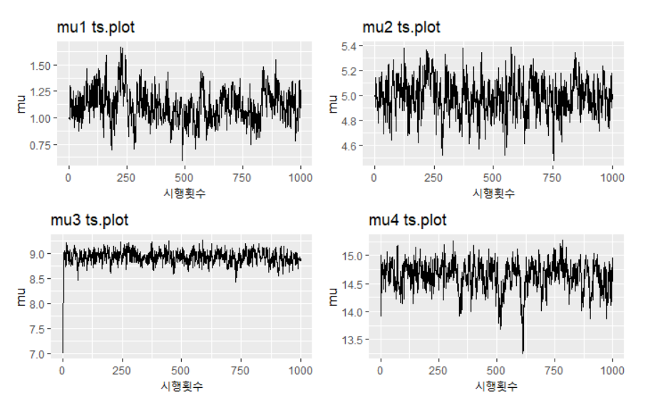
아래는 평균에 대한 시계열 그림이다.

p1 <- ggplot() + geom_line(aes(c(1:1000),mu_post[1:1000,1]))  + ggtitle("mu1 ts.plot") +xlab("시행횟수")+ylab("mu")
p2 <- ggplot() + geom_line(aes(c(1:1000),mu_post[1:1000,2]))  + ggtitle("mu2 ts.plot")+xlab("시행횟수")+ylab("mu")
p3 <- ggplot() + geom_line(aes(c(1:1000),mu_post[1:1000,3]))  + ggtitle("mu3 ts.plot")+xlab("시행횟수")+ylab("mu")
p4 <- ggplot() + geom_line(aes(c(1:1000),mu_post[1:1000,4]))  + ggtitle("mu4 ts.plot")+xlab("시행횟수")+ylab("mu")
grid.arrange(p1,p2,p3,p4,nrow=2)

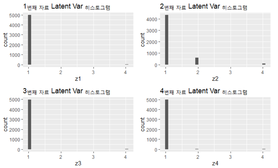
Gibbs Sampler를 통한 Latent Variable 추정은 z_post 객체에 저장되어 있다. 예를 들어 1~4번째 자료의 latent variable에 대한 추정 분포는 다음과 같다.

p2 <- ggplot() + geom_histogram(aes(z_post[5000:10000,1]))  + ggtitle("1번째 자료 Latent Var 히스토그램") + xlab("z1")
p3 <- ggplot() + geom_histogram(aes(z_post[5000:10000,2]))  + ggtitle("2번째 자료 Latent Var 히스토그램") + xlab("z2")
p4 <- ggplot() + geom_histogram(aes(z_post[5000:10000,3]))  + ggtitle("3번째 자료 Latent Var 히스토그램") + xlab("z3")
p5 <- ggplot() + geom_histogram(aes(z_post[5000:10000,4]))  + ggtitle("4번째 자료 Latent Var 히스토그램") + xlab("z4")
grid.arrange(p2,p3,p4,p5,nrow=2)

EM Algorithm 으로 Latent Variable 찾기

EM 알고리즘의 스텝은 다음과 같다.

log-likelihood 함수인 $log \ p(x,z \mid \theta)$를 구한다.
Q-function $\equiv E_{z}(log \ p(x,z \mid \theta))$를 찾는다.
Q-function을 최대화 시키는 $\theta$를 찾아 $\theta^{t+1}$로 둔다
2,3을 수렴할때 까지 반복한다.

1. log-likelihood 함수인 $log \ p(x,z \mid \theta)$를 구한다.

우선 1번을 하기 위해 likelihood 함수를 찾아보자. 데이터는 다음과 같은 분포를 따른다고 가정할 수 있다.

$Y_i \sim \sum^{4}_{k=1}\pi_kN(y_i;u_k,\tau_k)$

앞선 경우와 마찬가지로 k=4를 가정하면 Latent Variable은 $\theta ={ \mu_k,\tau_k, \pi_k \ ; k=1,2,3,4 }$에 의해 정해진다고 볼 수 있다. 따라서 다음과 같이 구할 수 있다.

$p(x,z \mid \theta) = p(x \mid z , \theta) p(z \mid \theta)$
$= \prod_i N(x_i;\mu_{z_i},\tau_{z_i})p(z_i|\theta)$ $= \prod_i \prod_k(\pi_k N(x_i;\mu_k,\tau_k))^{I(z_k=1)}$

$l(x,z \mid \theta)=\sum_i \sum _k[ I(z_i=k)(log \ \pi_k -\frac{1}{2}log \ \tau_k - \frac{1}{2 \tau_k}(x_i-\mu_k)^2)]$

2. Q-function $\equiv E_{z}(log \ p(x,z \mid \theta))$를 찾는다.

$Q(\theta \mid \theta^{t}) = E_{z}(l(x,z \mid \theta)) = \sum_i \sum _k[ I(\hat{z}_i=k)(log \ \pi_k -\frac{1}{2}log \ \tau_k - \frac{1}{2 \tau_k}(x_i-\mu_k)^2)]$

$\hat{z_i} = E[z_i \mid x,\theta^{t}] $ 앞서서 구한 $p(x,z \mid \theta^t)$의 꼴을 살펴보면 다음과 같이 구할 수 있다.
$z_i \mid x,\theta^t \sim Multi([\frac{\pi_k N(x_i;\mu_k,\tau_k))}{\sum_{p=1}^4(\pi_p N(x_i;\mu_p,\tau_p))}]_{k=1}^4)$

3. Q-function을 최대화 시키는 $\theta$를 찾아 $\theta^{t+1}$로 둔다

Q($\theta^{t+1} \mid \theta^t$)을 maximize 시키기 위해서 미분해서 0이 나오는 지점을 찾으면 다음과 같다.

$\frac{d}{d \mu_1}Q = \sum_i I(\hat{z_i}=1)\frac{1}{\tau_1}(x_i-\mu_1) = 0$

$\mu_1^{t+1} = \frac{\sum_i I(\hat{z_i}=1)x_i}{\sum_i I(\hat{z_i}=1)} = \bar{x}_1$

$\frac{d}{d \tau_1}Q = \sum_i -I(\hat{z_i}=1)[\frac{1}{2 \tau_1}-\frac{1}{2 \tau_1^2}(x_i-\mu_1)^2]=0$

$\tau_1^{t+1} = \frac{\sum_i I(\hat{z_1}=1) (x_i-\mu_1)^2}{\sum_i I(\hat{z_1}=1)} = S_1^2$

$\pi_1$에 대한 미분의 경우 $\sum_k\pi_k=1$이라는 제약이 있으므로 라그랑주를 취한 다시 구해줄 수 있다. 그결과는 다음과 같다.

$\pi_1^{t+1} = \frac{\sum \hat{z_1}}{n}$

이렇게 구한 이터레이션 폼을 이용하여 반복문을 짜주자

초기값 설정은 다음과 같이 해줬다.

iter = 10000

mu_current = c(1,5,9,11)
tau_current = c(1,1,1,1)
pi_current = c(0.25,0.25,0.25,0.25)

z_current = c()
for (i in 1:dim(data)[1]){
  
  density = c()
  
  for (k in 1:K){
    kprob = dnorm(data[i,2],mu_current[k],tau_current[k]^(0.5))*pi_current[k]
    density = append(density,kprob)
  }
  
  z_ind = c(1,2,3,4)[rank(density)==4]
  
  z_current = append(z_current,z_ind)
}

mu_em = mu_current
tau_em = tau_current
pi_em = pi_current
z_em = z_current

이제 최적화기법을 시행해줬다. 다음 시행과의 차이가 0.01이하 일시 얼리스탑을 할 수 있도록 코드를 설정해주었다.

for (it in c(1:iter)){

z_t1 = c()
for (i in 1:dim(data)[1]){
  
  density = c()
  
  for (k in 1:K){
    kprob = dnorm(data[i,2],mu_current[k],tau_current[k]^(0.5))*pi_current[k]
    density = append(density,kprob)
  }
  
  z_ind = c(1,2,3,4)[rank(density)==4]
  
  z_t1 = append(z_t1,z_ind)
}

mu_t1 = c()
for (k in c(1:K)){
  mu_part = mean(data[z_current == as.character(k),2])
  mu_t1 = append(mu_t1,mu_part)
}

tau_t1 = c()
for (k in c(1:K)){
  tau_part = sum((data[z_current == as.character(k),2]-mu_current[k])^2)/sum(z_current == as.character(k))
  tau_t1 = append(tau_t1,tau_part)
}

pi_t1 = c()
for (k in c(1:K)){
  pi_part = sum(z_current == as.character(k))/dim(data)[1]
  pi_t1 = append(pi_t1,pi_part)
}


mu_em = rbind(mu_em,mu_t1)
tau_em =rbind(tau_em,tau_t1)
pi_em =rbind(pi_em,pi_t1)
z_em =rbind(z_em,z_t1)

if ((abs(sum(mu_t1-mu_current))<abs(sum(mu_t1))*0.01)*(abs(sum(tau_t1-tau_current))<abs(sum(tau_t1))*0.01)*(abs(sum(pi_t1-pi_current))<abs(sum(pi_t1))*0.01) ==1){break}

mu_current = mu_t1
tau_current = tau_t1
pi_current = pi_t1
z_current = z_t1

}

알고리즘의 수렴정도를 보니 다음과 같았다.

p1 <- ggplot() + geom_line(aes(c(1:dim(mu_em)[1]),mu_em[,1]))  + ggtitle("mu1 ts.plot") +xlab("시행횟수")+ylab("mu1")
p2 <- ggplot() + geom_line(aes(c(1:dim(mu_em)[1]),mu_em[,2]))  + ggtitle("mu2 ts.plot")+xlab("시행횟수")+ylab("mu2")
p3 <- ggplot() + geom_line(aes(c(1:dim(tau_em)[1]),tau_em[,1]))  + ggtitle("tau1 ts.plot")+xlab("시행횟수")+ylab("tau1")
p4 <- ggplot() + geom_line(aes(c(1:dim(pi_em)[1]),pi_em[,1]))  + ggtitle("pi1 ts.plot")+xlab("시행횟수")+ylab("pi1")
grid.arrange(p1,p2,p3,p4,nrow=2)

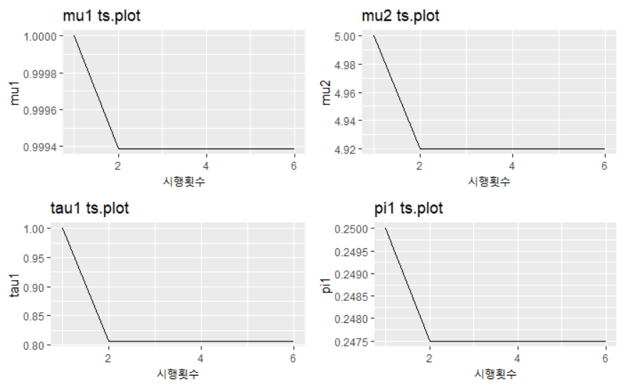
gibbs sampler에 비해 훨신 적은 숫자로 수렴하는 것에 성공했다.

두 알고리즘 비교

Gibbs Sampler와 EM algorithm으로 추정한 군집 모수들은 다음과 같다.

clt_mean = rbind(mu_t1,apply(mu_post[5000:10000,],2,mean))
clt_var = rbind(tau_t1,apply(tau_post[5000:10000,],2,mean))
z_index = rbind(z_t1,apply(z_post[5000:10000,],2,mean))
clt_mean

두 알고리즘의 결과물 평균은 거의 흡사하다고 말할 수 있다.

다음으로 두 알고리즘에서 나온 결과물으로 히스토그램을 다시 그려보았다.

Gibbs Sampler의 히스토그램

result = data.frame(cbind(data["x"],"gibbs" = as.factor(round(apply(z_post[5000:10000,],2,mean))),"em"=as.factor(z_current)))
result %>%
 ggplot(aes(x,fill=gibbs))+geom_histogram()

EM Alogorithm의 히스토그램

result %>%
 ggplot(aes(x,fill=em))+geom_histogram()

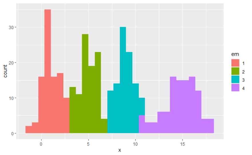
거의 흡사하게 잘 분류해낸것을 볼 수 있다.

Twitter Facebook LinkedIn

[Bayesian Inference] GMM 모수 추정 실습

H.G Min

Bayesian Statistics

개요

Gibbs Sampler로 Latent Variable 찾아내기

1. $\mu,\tau$의 FCD 체크하기

2. $\pi,z_i$의 FCD 체크하기

EM Algorithm 으로 Latent Variable 찾기

1. log-likelihood 함수인 $log \ p(x,z \mid \theta)$를 구한다.

2. Q-function $\equiv E_{z}(log \ p(x,z \mid \theta))$를 찾는다.

3. Q-function을 최대화 시키는 $\theta$를 찾아 $\theta^{t+1}$로 둔다

두 알고리즘 비교

You May Also Enjoy

[Paper Review] Dimensionality Reduction as Probabilistic Inference

[Paper Review] Dimensionality Reduction as Probabilistic Inference

계속 쓰는 시

6월의 시