title: [Basic of Quantum Computer] Part 5. Quantum Phase Estimation and Quantum Distance Measure categories: [Quantum] tags: [Quantum Computer] excerpt: Quantum Phase Estimation와 Quantum State Distance Measure sidebar:
- title: “Quantum Computing” image: /assets/img/quantum.png image_alt: “image” nav: Quantum_eng author_profile: False —
$\def\ket#1{\mid #1 \rangle} \def\inner#1{\langle #1 \rangle}$
Chapter 4. Quantum Phase Estimation and Quantum Distance Measure
Let’s see the second important quantum routine.
1. Quantum Phase Estimation
Quantum gates are expressed by the matrix. But the norms of each Qubit always have to be one before and after it passes the operator. This is because the sum of all probabilities have to be one.
Therefore, we can develop the following expression.
$\inner{\phi\mid A\mid \phi}=1$ for all $\ket{\phi} $ where $\inner{\phi \mid \phi}=1$
There is a quadratic form theorem that the quadratic form’s spectrum is always in the range between minimum of the eigenvalue and maximum of the eigenvalue.
It can be expressed as follow
$\min_{v \mid v^tv =1}( \mid v^t A v \mid)=\lambda_1 , \max_{v \mid v^tv =1} (\mid v^t A v \mid) = \lambda_n $
Therefore, we can say that absolute value of all of eigenvalue of the A is 1 and we can generalized them as follow
$\lambda =e^{2\pi \psi i} \mbox{ where } \psi \in [0,1)$
Quantum Phase Estimation is estimating eigenvalue by estimating phase of a certain operator.
Application of the Unitary Matrix
If we set the eigenvalue of $U$ as $e^{2 \pi \psi i}$ and eigenvector of U as $\ket{\psi}$, then we can get
$U \mid \psi \rangle = e^{2\pi \psi i }\mid \psi \rangle$
If we apply them, then we can generalize them with the case of $2^m$ as follow
$U \mid \Psi \rangle = e^{2 \pi \psi i}\mid \Psi \rangle$
$U^2 \mid \Psi \rangle = U e^{2\pi \psi i}\mid \Psi \rangle = e^{2\times2\pi \psi i}\mid \Psi \rangle$
$\cdots$
$U^{2^{j}} \mid \Psi \rangle= e^{2^{j+1}\pi \psi i}\mid \Psi \rangle$
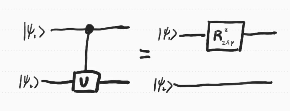
Therefore, if the U is applied to an eigenvector, then it works the same way with $U=e^{2 \pi \psi i}I$. So we can simplify it as follows.
$e^{2\pi \psi i} \left[ \begin{array}{cc} 1 & 0 \\ 0 & 1 \end{array}\right] = \left[ \begin{array}{cc} e^{2\pi \psi i} & 0 \\ 0 & e^{2\pi \psi i} \end{array}\right] $
pf)
Let $\ket \psi_1 = a \ket 0+ b \ket 1$
then $cU(\ket {\Psi_1},\ket {\Psi_2}) = a\ket 0\otimes \ket {\Psi_2}+b\ket 1 \otimes U \ket {\Psi_2} \\ \qquad \qquad \qquad \ = a\ket 0\otimes \ket {\Psi_2}+b\ket 1 \otimes e^{2 \pi \Psi i } \ket {\Psi_2} \\ \qquad \qquad \qquad \ =(a \ket 0 +be^{2 \pi \Psi i}\ket 1 )\otimes \ket {\Psi_2} \\ \qquad \qquad \qquad \ =R_{2 \pi \psi} \ket {\Psi_1} \otimes \ket{ \Psi_2} $
Quantum Phase Estimation Circuit
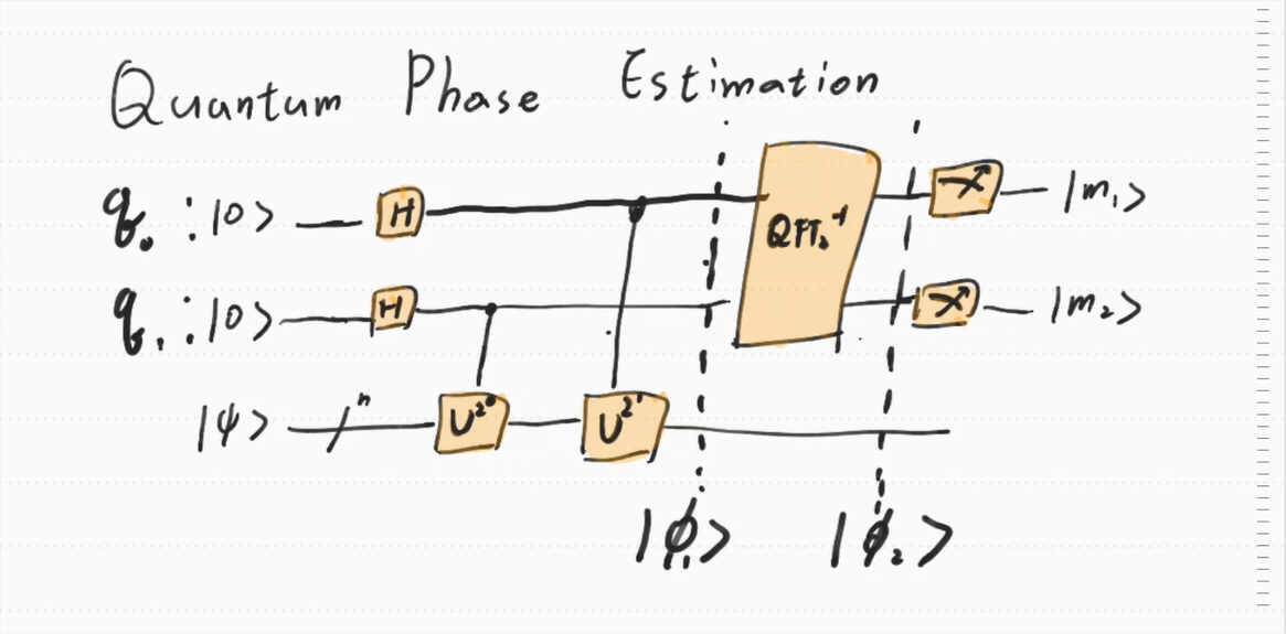
The circuit of quantum phase estimation(;QPE) is below.
This is the QPE of a 2-qubit quantum gate. Let’s track it down
First of all, let’ see $q_0$ and $q_1$ to check the state of $\ket{\phi_1}$
In the case of $q_0$,
$cU^{2^1}(H\ket 0 , \ket \Psi) = cU^{2^1}(\frac{1}{\sqrt{2}}(\ket 0 + \ket 1 ),\ket \Psi) \\ \qquad \qquad \qquad \quad \ = \frac{1}{\sqrt{2}}(\ket 0 \ket \Psi + \ket 1 U^{2^1}\ket \Psi) \\ \qquad \qquad \qquad \quad \ =\frac{1}{\sqrt{2}}(\ket 0 \ket \Psi + \ket 1 e^{2^ 2 \pi \psi i }\ket \Psi) \\ \qquad \qquad \qquad \quad \ = \frac{1}{\sqrt{2}}(\ket 0 + e^{2 \pi 2^1 \psi i }\ket 1 ) \otimes\ket \Psi)$
$q_1$ can be inferred as follows.
$cU^{2^0}(H\ket 0 , \ket \Psi)= \frac{1}{\sqrt{2}}(\ket 0 + e^{2 \pi 2^0 \psi i }\ket 1 ) \otimes\ket \Psi)$
Therefore, $\ket{\phi}_1$ is as follows.
$\ket \phi_1 = \frac{1}{2}(\ket 0 + e^{2 \pi 2^1 \psi i }\ket 1 ) \otimes (\ket 0 + e^{2 \pi 2^0\psi i }\ket 1 ) \otimes \ket \Psi \\ \quad \ \ = \frac{1}{2}(\ket{00}+e^{2\pi2^0\psi i}\ket{01}+e^{2 \pi 2^1 \psi i }\ket{10}+e^{2 \pi (2^2-1) \psi i}\ket{11}) \otimes \ket \Psi\\ \quad \ \ =\frac{1}{\sqrt{2}^2} \sum_{j=0}^{2^2-1}e^{2\pi j \psi i} \ket j_2 \otimes \ket \Psi$
Next part is the Inverse QFT gate. Let’s see how it works.
For the $N=2^n$, inverse - QFT works as follows.
$\ket \chi = \sum_{j=0}^{2^2-1}a_j\ket j _2$
$QFT^{-1}(\ket \chi)=\frac{1}{\sqrt{2^2}}\overset{2^2-1}{\underset{j=0}{\sum}}\overset{2^2-1}{\underset{k=0}{\sum}}a_ke^{-\frac{2 \pi ijk}{2^2}} \ket j _2$ ($a_k = \frac{1}{\sqrt{2^2}}e^{2 \pi j \psi i}$)
Therefore, $\ket{\phi_2} = QFT^{-1}(\frac{1}{\sqrt{2}^2} \sum_{j=0}^{2^2-1}e^{2\pi j \psi i} \ket j_2) \otimes \ket{\Psi_2}$is below
$QFT^{-1}(\frac{1}{\sqrt{2}^2} \sum_{j=0}^{2^2-1}e^{2\pi j \psi i} \ket j_2) = \frac{1}{2^2}\overset{2^2-1}{\underset{j=0}{\sum}}\overset{2^2-1}{\underset{k=0}{\sum}} e^{2 \pi j \psi i} e^{-\frac{2 \pi ijk}{2^2}} \ket j _2 \\ \qquad\qquad\qquad\qquad\qquad\qquad\quad= \frac{1}{2^2}\overset{2^2-1}{\underset{j=0}{\sum}}\overset{2^2-1}{\underset{k=0}{\sum}} e^{-\frac{2 \pi k i}{2^2} (j- 2^2\psi) } \ket j _2$
If we interpret the result, then we can say that the amplitudes of $\ket{j}_2$ are $\frac{1}{2^2}\overset{2^2-1}{\underset{k=0}{\sum}} e^{-\frac{2 \pi k i}{2^2} (j- 2^2\psi) }$
We can get the following result with generalizing it as $2^m$- qubit
the amplitude of $\ket {j}$ : $\frac{1}{2^m}\overset{2^m-1}{\underset{k=0}{\sum}} e^{-\frac{2 \pi k i}{2^m} (j- 2^m\psi) }$
How can we interpret the result?
Above amplitude is sample mean value of random variable k, so it is the estimator of $E(e^{-\frac{2 \pi k i}{2^m} (j- 2^m\psi) })$ and $p(j)$
Therefore, $\hat{p}(j)= \mid \frac{1}{2^m}\overset{2^m-1}{\underset{k=0}{\sum}} e^{-\frac{2 \pi k i}{2^m} (j- 2^m\psi) } \mid ^2 = \frac{1}{2^{2m}}\mid\overset{2^m-1}{\underset{k=0}{\sum}} e^{-\frac{2 \pi k i}{2^m} (j- 2^m\psi) } \mid ^2$
It takes its highest value at $j=2^m \psi$ which means that if we iterate the circuit, then mode of the results is $2^{m} \psi$ and we can estimate $\psi$ as $\frac{j}{2^m}$
Now, see j
- j takes value between $0$ and $2^m -1$ so $\frac{j}{2^m}$ lies in $(0, \frac{2^m -1}{2^m})$. $\psi$ represent the phase
- j gets its name by assigning a combination of computational basis. For example, with 5-qubit, we can name each basis as follow $\ket{j}$
$\ket{0} = \ket {00000}$
$\ket{1} = \ket{00001}$
$\ket{2} = \ket{00010}$
$\ket{3} = \ket{00011}$
$\ket{4} = \ket{00100}$
…
$\ket{30} = \ket{11110}$
$\ket{31} = \ket{11111}$
Let’s change them as binary expression
$0 = 0_{(2)}$
$1 = 1_{(2)}$
$2 = 10_{(2)}$
$3 = 11_{(2)}$
…
$31 = 11111_{(2)}$
$32 =100000_{(2)}$
Each pair exactly matches with the above naming. Therefore, the $\frac{j}{2^m}$ have the following meaning.
$0.b_1b_2b_3b_4…b_m$ $(b_i \in {0,1} \quad \forall i)$ ($b_i$is observation of $\ket {q}_{2^m}$)
For example, assume that we get the following value as mode by iterating the circuit multiple times.
$\ket{110010110011}$
Then the estimate of the eigenvalue is $0.110010110011_{(2)}$
The eigenvalues are usually infinite values, so QPE estimates the eigenvalues in $log_{10}(2^{-m})$ digit. Therefore, there are some errors which can be lessened by iteration. That is, by increasing the number of the iteration and m-qubit, we can promote the estimative power.
Some people might wonder why we use eigenvectors even though the purpose of the circuit is to find eigenvalues. This is because any random vector can be analyzed by the linear combination of eigenvalues as follows $\ket{b} = \sum \lambda_i \ket{\psi_i}$.
By assuming them, we can make some practical algorithm like HHL algorithm for linear solver
2. Quantum Distance Measure
Now, let’s think about two states $\ket{\psi _\alpha}, \ket{\psi_b}$. There are quantum circuits which can be good for measuring them.
Standard metric unit L2-distance can be measured as follows.
$\mid \ket{\psi_\alpha} - \ket{\psi_{\beta}}\mid_2^2 = (\ket{\psi_\alpha} - \ket{\psi_{\beta}})^t(\ket{\psi_\alpha} - \ket{\psi_{\beta}}) \\ \qquad\qquad \qquad= \langle \psi_{\alpha},\psi_\beta \rangle - \langle \psi_{\alpha},\psi_\alpha \rangle-\langle \psi_{\alpha},\psi_\beta \rangle+\langle \psi_{\beta},\psi_\beta \rangle \\ \qquad\qquad \qquad= 2-2RE{\langle \psi_{\alpha},\psi_\beta \rangle}$
Quantum state can make the state using the operator like $\ket {\psi_\alpha} = U_\alpha \ket 0 , \ket {\psi_\beta} = U_\beta \ket 0$
We can calculate them with Hadamard test and SWAP test
Hadamard Test
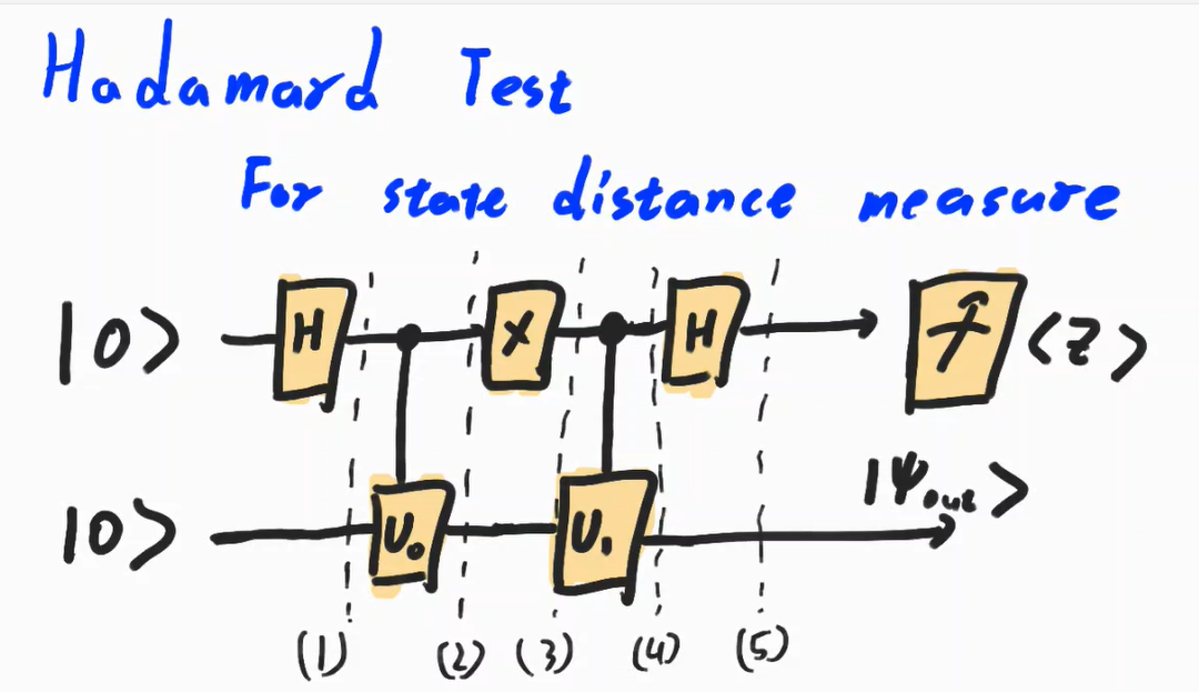
Circuit of Hadamard Test is like below
Let’s track it down.
-
$\ \ket{\psi_1} = \frac{1}{\sqrt 2}( \ket 0 + \ket 1) \ket 0 \\ \qquad \propto \ket {00} + \ket {10}$
-
$\ \ket {\psi_2} = cU_{\alpha} (\ket {00} + \ket {10})\\ \qquad = \ket{00}+\ket{1 \ \psi_\alpha}$
-
$\ \ket{\psi_3} = \ket{10}+\ket{0\psi_\alpha}$
-
$\ket{\psi_4} = cU_{\beta}(\ket{10}+\ket{0\psi_\alpha}) \\ \qquad = \ket{1 \psi_\beta} + \ket{0\psi_\alpha}$
-
$\ \ket{\psi_5} = (\ket{0} + \ket{1})\ket{\psi_\alpha} +(\ket 0 - \ket 1)\ket {\psi_\beta} \\ \qquad \propto \frac{1}{2}\ket{0}(\ket{\psi_\alpha}+\ket{\psi_\beta})+\frac{1}{2}\ket{1} (\ket{\psi_\alpha} - \ket{\psi_\beta}) $
-
Measure :
$p(0) = \frac{1}{2}^2\mid\ket{\psi_\alpha}+\ket{\psi_\beta}\mid^2 = \frac{1}{2} + \frac{1}{2}Re{\langle \psi_\alpha \mid \psi_{\beta} \rangle}$
$p(1) = \frac{1}{2}^2\mid\ket{\psi_\alpha}+\ket{\psi_\beta}\mid^2 = \frac{1}{2} - \frac{1}{2}Re{\langle \psi_\alpha \mid \psi_{\beta} \rangle}$
That is, we can measure the metric by iterating the circuit multiple times and observing the ratio of zero and one.
SWAP Test
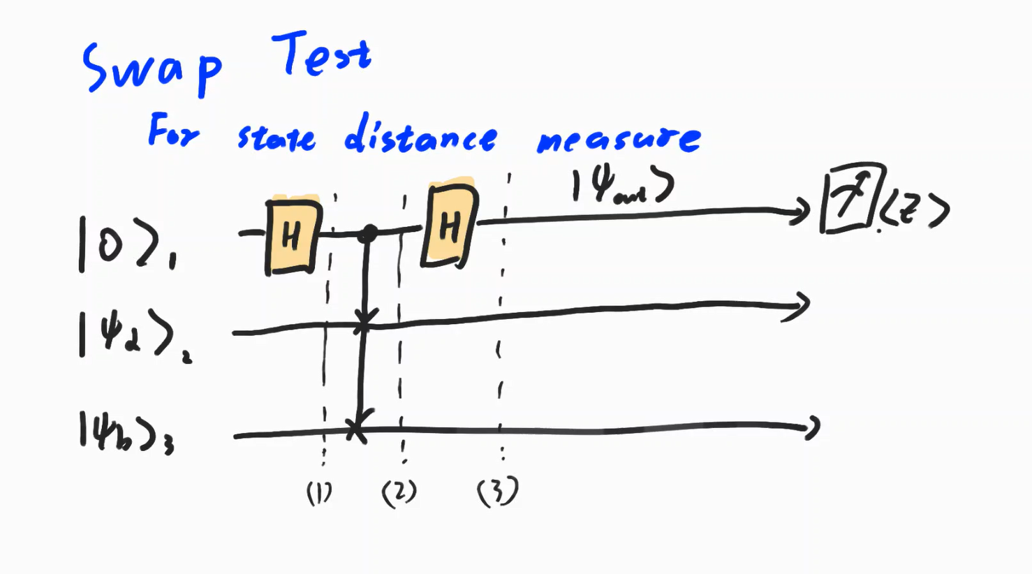
The Swap test have almost similar role with Hadamard test
-
$\ket{\psi_1} = (\ket 0 + \ket 1)\ket{\psi_\alpha \psi_\beta}$
-
$\ket{\psi_2} = Fredkin(\ket{\psi_1}) \\ \ \quad = \ket{0\psi_\alpha\psi_\beta}+\ket{1\psi_\beta\psi_\alpha}$
-
$\ket{\psi_3} = \ket{0}(\ket{\psi_\alpha \psi_\beta}+\ket{\psi_\beta \psi_\alpha}) + \ket{1}(\ket{\psi_\alpha \psi_\beta}-\ket{\psi_{\beta}\psi_{\alpha}} $
-
Measure:
$p(0) = \frac{1}{2} + \frac{1}{2}\mid\langle \psi_\alpha, \psi_ \beta \rangle\mid^2$
$p(0) = \frac{1}{2} - \frac{1}{2}\mid\langle \psi_\alpha, \psi_ \beta \rangle\mid^2$
We can measure it like above.
Sutor, R. (2019). Dancing With Qubits. Birmingham,UK:Packt
Bernhardt, C. (2019). Quantum computing for everyone. Boston, Massachusetts:The MIT Press
 pf)
Let $\ket \psi_1 = a \ket 0+ b \ket 1$
then $cU(\ket {\Psi_1},\ket {\Psi_2}) = a\ket 0\otimes \ket {\Psi_2}+b\ket 1 \otimes U \ket {\Psi_2} \\ \qquad \qquad \qquad \ = a\ket 0\otimes \ket {\Psi_2}+b\ket 1 \otimes e^{2 \pi \Psi i } \ket {\Psi_2} \\ \qquad \qquad \qquad \ =(a \ket 0 +be^{2 \pi \Psi i}\ket 1 )\otimes \ket {\Psi_2} \\ \qquad \qquad \qquad \ =R_{2 \pi \psi} \ket {\Psi_1} \otimes \ket{ \Psi_2} $
Quantum Phase Estimation Circuit
The circuit of quantum phase estimation(;QPE) is below.
 This is the QPE of a 2-qubit quantum gate. Let’s track it down
First of all, let’ see $q_0$ and $q_1$ to check the state of $\ket{\phi_1}$
In the case of $q_0$,
$cU^{2^1}(H\ket 0 , \ket \Psi) = cU^{2^1}(\frac{1}{\sqrt{2}}(\ket 0 + \ket 1 ),\ket \Psi) \\ \qquad \qquad \qquad \quad \ = \frac{1}{\sqrt{2}}(\ket 0 \ket \Psi + \ket 1 U^{2^1}\ket \Psi) \\ \qquad \qquad \qquad \quad \ =\frac{1}{\sqrt{2}}(\ket 0 \ket \Psi + \ket 1 e^{2^ 2 \pi \psi i }\ket \Psi) \\ \qquad \qquad \qquad \quad \ = \frac{1}{\sqrt{2}}(\ket 0 + e^{2 \pi 2^1 \psi i }\ket 1 ) \otimes\ket \Psi)$
$q_1$ can be inferred as follows.
$cU^{2^0}(H\ket 0 , \ket \Psi)= \frac{1}{\sqrt{2}}(\ket 0 + e^{2 \pi 2^0 \psi i }\ket 1 ) \otimes\ket \Psi)$
Therefore, $\ket{\phi}_1$ is as follows.
$\ket \phi_1 = \frac{1}{2}(\ket 0 + e^{2 \pi 2^1 \psi i }\ket 1 ) \otimes (\ket 0 + e^{2 \pi 2^0\psi i }\ket 1 ) \otimes \ket \Psi \\ \quad \ \ = \frac{1}{2}(\ket{00}+e^{2\pi2^0\psi i}\ket{01}+e^{2 \pi 2^1 \psi i }\ket{10}+e^{2 \pi (2^2-1) \psi i}\ket{11}) \otimes \ket \Psi\\ \quad \ \ =\frac{1}{\sqrt{2}^2} \sum_{j=0}^{2^2-1}e^{2\pi j \psi i} \ket j_2 \otimes \ket \Psi$
 Let’s track it down.
 The Swap test have almost similar role with Hadamard test