
1. Barrier Method
By using Gradient Descent or Newton Raphson Method, We can solve unconstrained convex optimization problems very easily. However, If our problem has inequality constraints, then the problem becomes much more difficult. For gradient descent, we have to use projected GD which could be hard to implement for some problem.
For Newton’s method, we can use a much more elegant method to solve the problem. There are two famous methods: Barrier Method and Primal-Dual Interior Point Method. In this posting, we’ll see the Barrier Method.
Assume the following canonical convex optimization problem.
\[\underset{x}{ \min} f(x) \\ \mbox{ s.t. } \begin{cases}h_i(x)\leq 0 , i=1,2,...,m \\ Ax =b \end{cases}\]For the problem, we’ll gonna define $\phi(x) = - \underset{i=1}{\overset{m}{\sum}} \log ( -h_i (x))$ which is called as log barrier function. For it, the domain of $\phi(x)$ is ${x : h_i(x)<0}$ which is a strictly feasible set. Therefore, strong duality which means that the gap between primal and dual is zero holds for the problem by Slater’s condition.
When we directly inject the constraints to problem, then it becomes as follow
\[\underset{x}{\min} f(x) + \underset{i=1}{\overset{m}{\sum}} I_{\{h_i(x) \leq 0 \}}(x)\]Because the indicator functions can not be differentiable, so we can use the log barrier function instead.
\[\underset{x}{\min} f(x) - \frac{1}{t} \underset{i=1}{\overset{m}{\sum}} \log ( -h_i (x))\]Let’s compare them.
- $\underset{i=1}{\overset{m}{\sum}} I_{{h_i(x) \leq 0 }}(x)$ would be infinity if one of the $h_i(x)$ becomes positive
- $-\frac{1}{t} \underset{i=1}{\overset{m}{\sum}} \log ( -h_i (x))$would be close to infinity if one of the $h_i(x)$ goes to zero
- $\underset{i=1}{\overset{m}{\sum}} I_{{h_i(x) \leq 0 }}(x)$ would be zero if all of the $h_i(x)$ are negative
- $-\frac{1}{t} \underset{i=1}{\overset{m}{\sum}} \log ( -h_i (x))$would be $\frac{c}{t}$ if all of the $h_i(x)$ are negative and become zero as $t$ increases
Because two functions work in the similar way, so with delicate handling with t, we can substitute it.
For the log barrier function, we can get derivatives as follows.
- $\phi (x) = -\underset{i=1}{\overset{m}{\sum}} \log (- h_i(x))$
- $\nabla \phi (x) = -\underset{i=1}{\overset{m}{\sum}} \frac{1}{h_i(x)}\nabla h_i(x))$
- $\nabla^2 \phi (x) = \underset{i=1}{\overset{m}{\sum}} \frac{1}{h_i^2(x)}\nabla h_i(x)\nabla h_i(x)^t -\underset{i=1}{\overset{m}{\sum}} \frac{1}{h_i (x)}\nabla^2 h_i(x)$
2. Central Path
Even though we can use the log barrier method, the two problems are essentially different. Therefore, we have to use a special routine called the central path.
Assume barrier problem
\[\underset{x}{\min} t f(x) + \phi(x) \\ \mbox{ s. t. } Ax =b\]This problem highly depends on it. Therefore, we have to define the solution as $x^{\ast}(t)$.
Let’s figure it out with the Dual problem.
$\underset{x}{\min} t f(x) - \underset{i=1}{\overset{m}{\sum}} \log (-h_i(x)) \mbox{ s.t. } Ax=b$
Let’s solve it with KKT conditions.
$\Rightarrow t \nabla f(x^{\ast}(t)) - \underset{i=1}{\overset{m}{\sum}} \frac{1}{h_i(x^{\ast}(t))}\nabla h_i(x^{\ast}(t))+A^tw =0 \mbox{ (Stationarity)}$
$Ax^{\ast}(t) =b , h_i(x^{\ast}(x)) <0 \mbox{ (Feasibility)}$
And let’s see the KKT condition of the original problem.
$\underset{x}{\min} f(x) \mbox{ s.t. } h_i(x) \leq 0 \mbox{ and } Ax =b$
$L(x,u,v) = f(x) + \underset{i=1}{\overset{m}{\sum}} u_i h_i(x) + v^t (Ax-b)$
$\Rightarrow \nabla f(x) + \underset{i=1}{\overset{m}{\sum}}u_i \nabla h_i(x) + A^tv =0$
$\Rightarrow t\nabla f(x) + \underset{i=1}{\overset{m}{\sum}}tu_i \nabla h_i(x) + tA^tv =0 $
The solution is $(x,u,v) = (x^{\ast}(t),u^{\ast}(t),v^{\ast}(t)) = (x^{\ast}(t),-\frac{1}{t h_i(x^{\ast}(t))},\frac{w}{t})$
$w$ and $x^{\ast}$ are the same variable with a barrier problem. So we can see the connection between these two problems.
Moreover we can see the duality gap as follows.
$\underset{x}{\min} L(x^{\ast}(t) , u^{\ast}(t),v^{\ast}(t)) = f(x^{\ast}(t)) + \underset{i=1}{\overset{m}{\sum}} u_i^{\ast}(t) h_i(x^{\ast}(t)) + v^{\ast}(t)^t (Ax^{\ast}(t)-b)$
$= f(x^{\ast}(t))-\frac{m}{t} \leq f^{\ast}$
$\Rightarrow f(x^{\ast}(t))-f^{\ast} \leq \frac{m}{t}$
So as it goes to infinity, the duality gap becomes zero.
We can summarize the above result as follow.
Perturbed KKT Condition
Stationarity $: \nabla f(x) + \underset{i=1}{\overset{m}{\sum}}u_i \nabla h_i(x) + A^tv =0 $
Complementary Slackness : $u_i \cdot h_i (x) = - \frac{1}{t}$
Primal Feasibility : $h_i(x) \leq 0 ,Ax =b$
Dual Feasibility : $u_i\geq 0$
We can say that the Barrier method is equal to solving the above problem.
Barrier Method
- For fixed $t^{(0)}, \mu >1$, Solve the problem with NM ; $x^{(0)}= x^{\ast}(t)$
- $t =t ^{(k)}, x_{init} = x^{k-1}$ Solve the problem with NM ; $x^{(k)} = x^{\ast}(t)$
- Check if $m/t \leq \epsilon$ and if it is true, then stop else if False, $t^{(k+1)} = \mu t$
If the $\mu$ and $t^{(0)}$ are too small, then we have to take more than 2,3 steps and if they are too big, then we have to take more 1 step.
Convergence Analysis
The barrier method after k centering steps satisfies $f(x^{(k)}) -f^{\ast} \leq \frac{m}{\mu^{k}t^{(0)}}$
So the problem takes $O(\log \frac{1}{\epsilon})$ step.
3. Visualization of Barrier Method
If we see the form of barrier problem, then we can notice that it is a combination of constraints function and objective functions. The ratio of the combination is determined by a constant t. If t is small, then the effects of constraints function dominates an entire shape of function. If t is large, then the effects of objective function dominate the shape of function. Let’s see the figure below.
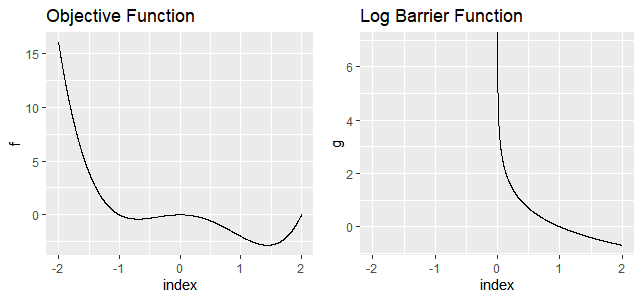
The left function is the polynomial function$(f(x) = x^2(x-2)(x+1))$ and the right function is the log barrier function for simple constraints ($-\log x ;x>0$).
So the problem would be as follows.
\[\underset{x}{\min} \quad x^2(x-2)(x+1) \\ \mbox{ s.t. }\quad \quad x>0\]The shapes of the log barrier problems which take t as 0.1,1,10 are as follow
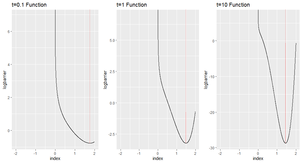
The red line indicates optima. As we can see, all functions succeed to make the shape restricted to positive value. At the small t, the shape resembles the constraint function. At the large t, the shape resembles the original function which satisfies the constraint.
But if you carefully see the plot, then you can notice that optima values represented by the red line are different along t. Specifically, each red line indicates 1.76,1.49,1.44. The true optima is 1.443. So we can observe that as t increases, the barrier optima reaches to true optima.
Boyd,S. & Vandenberghe, L. (2004) Convex Optimization.Cambridge, UK: Cambridge Press
Tibshirani,R. “Barrier Method” Convex Optimization, Oct. 2019, Carnegie Mellon University, Pittsburgh