
In this post, we’ll see the mathematical property of combination and eigenvalues. The combination is one of the most important parts of probability theory and the eigenvalue is most important concepts of the matrix theory.
There seems little connections between two concepts, but it proved that the combinatorics and matrix theory have deep connection. We’ll not gonna see this connection but if I study enough, maybe I can handle it somehow.
1. Stirling’s Formula
The term \(n!\) is most fundamental term of the combinatorics. However, although the term $n! = n\times (n-1)\times (n-2) \times (n-3)…\times 2 \times 1$ looks simple, but it is hard to handle its mathematical properties such as derivatives or integral.
Therefore, we need tractable representation replacing the term. The Stirling’s Formula implies the approximate behavior of factorial \(n!\) when the \(n\) becomes large.
Definition [Stirling’s Formula]
\[n! = (1+o(1))\sqrt{2\pi n} n^n e^{-n}\]
The book develop the approximation of the \(n!\) by gradually shrink the range of estimation. Let’s follow the procedure.
First of all, we can use the Taylor’s Expansion of \(e^{n}\). The Taylor’s expansion of \(e^{n}\) is \(1+n+\frac{1}{2!}n^2 +....+\frac{1}{n!}n^n+...\) Because \(n>0\), we can see that \(e^{n} \geq \frac{n^n}{n!}\) and \(n! \geq n^n e^{-n}\). And it is obvious that \(n^ne^{-n}\leq n!\leq n^n\).
We can get interval estimatior \([n^ne^{-n},n^n]\). However, the range of the interval is \(n^n(1-e^{-n})\) which is too big. For example, let’s see the \(n=5\) case. The exact value of \(5!\) is \(120\). The interval is \([21,3125]\) and the range is \(3101\). So we can know that it is not good estimator.
Secondly, we can use Riemann Integral Test which states that \(\int_{1}^n f \leq \sum_{i=1}^n f(i) \leq f(1)+\int_{1}^n f\).
By taking logarithm, we can see that \(\log n! = \sum_{m=1}^n \log m\). With the integral test, the inequality \(\int_{1}^n \log x dx \leq \sum_{m=1}^n \log m \leq \int_{1}^n \log x dx\).
By solving the integral with integration by part and applying exponential, we can get inequality \(en^ne^{-n} \leq n! \leq en\times n^n e^{-n}\) and interval estimator \([n^n e^{1-n},n^{n+1}e^{1-n}]\). Let’s apply it with \(n=5\). Then we can get the estimation \([57,286]\). It is much more exact interval then the first one, but we can do it better.
The third method is using Trapezoid Rule which is numerical integration methods states that \(\int_m^{m+1} f(x) dx = \frac{1}{2}f(m) +\frac{1}{2}f(m+1) + \epsilon_m\) where \(\epsilon_m \sim f''(m)\). In this case, \([log(x) ]'' \mid_{x=n} = O(\frac{1}{n^2})\) and \(\int_{m}^{m+1} \log x dx = \frac{1}{2}\log m + \frac{1}{2}\log (m+1) +\epsilon_m\).
By adding up, we can get \(\sum_{m=1}^n \epsilon_m = C + O(1/n),\int_{1}^n \log x dx = \sum_{m=1}^n \log m -\frac{1}{2}\log n +C + O(1/n)\). Therefore, we can get the estimator with big \(O\) notation as \(n! = (1+O(1/n))e^{1-C}\sqrt{n}n^n e^{-n}\).
Finally, to get more precise \(C\), we can use gamma function which is a result of the Stirling’s Formula. The gamma function is generalized version of factorial having domain in positive real number. It is \(\gamma(n) = \int_{0}^{\infty} t^{n-1} e^{-t}dt\) and if \(n \in \mathbb{N}\), \(\gamma(n)=(n-1)!\). We can expand the gamma function as follow.
\[n! = \int_{0}^{\infty}t^n e^{-t}dt\] \(= \int_{-n}^{\infty} (n+s)^ne^{-n-s}dsd\) (by substitute \(t=n+s\))
\(= n^n e^{-n}\int_{-n}^{\infty} (1+\frac{s}{n})^ne^{-s} ds\)
\(= n^n e^{-n}\int_{-n}^{\infty} exp(n \log (1+\frac{s}{n})-s) ds\)
\(= \sqrt{n}n^ne^{-n}\int_{-\sqrt{n}}^{\infty} \exp(n \log ( 1+ \frac{x}{\sqrt{n}})-\sqrt{n}x)dx\) (by substitute \(s=\sqrt{n}x\)) ——(A)
With Taylor expansion, we can get \(n \log (1+\frac{x}{\sqrt{n}}) = \sqrt{n}x -\frac{x^2}{2}-\frac{x^3}{3\sqrt{n}}...\) and therefore \(\exp(n\log(1+\frac{x}{\sqrt{n}})-\sqrt{n}x) \rightarrow \exp(-\frac{x^2}{2}), \forall x \in (0,\infty)\) as \(n \rightarrow \infty\). ——–(B)
And set \(f(x) = n \log (1+ \frac{x}{\sqrt{n}})\) and \(f(0)=0,f'(0)=\sqrt{n},f''(x) = -\frac{1}{(1+x/\sqrt{n})^2}\). Then we can get following result.
\[\int_{0}^{x}\frac{x-y}{1+y/\sqrt{n}}dy =\int_{0}^{x} f''(y)(x-y)dy\] \(= -x f'(x)+xf'(0)+\int_{0}^{x}yf''(y)dy\)
\(=-x f'(x)+xf'(0)+xf'(x)-f(x)+f(0)\)
\(=n\log(1+\frac{x}{\sqrt{n}})-\sqrt{n}x\)
It gives us the bound \(n \log (1+\frac{x}{\sqrt{n}})-\sqrt{n}x \leq \min(-cx^2,-cx\sqrt{n})\) ——–(C)
By (B) and (C), we can use the dominated convergence theorem \(\int_{-\sqrt{n}}^{\infty} \exp(n \log(1+\frac{x}{\sqrt{n}})-\sqrt{n}x)dx \rightarrow \int_{-\infty}^{\infty} \exp (-x^2/2)dx = \sqrt{2\pi}\)
Applying the result in (A), we can get the Stirling’s formula \(n! = (1+o(1))\sqrt{2\pi n}n^n e^{-n}\).
If we apply them with \(n=5\), we can get the estimation \((1+o(1))118\) which is much more similar with true value \(5! =125\). If we apply it with more large number such as 20, the exact values of it is \(2.432902 \times 10^{18}\) and Stirling’s formula givers us \(2.422787\times 10^{18}\) (Calculated with R program using log techniques \(\exp (\sum log (x))\)). Therefore, we can observe that our estimator works quite well.
By using the Stirling’s Formula, we can derive Entropy formula.
Entropy Formula
\(\left(\begin{array}{c} n \\ m\end{array}\right) = \exp [(h(\gamma)+o(1))n]\) where \(h(\gamma)\) is the entropy function \(h(\gamma) := \gamma \log \frac{1}{\gamma} +(1-\gamma)\log \frac{1}{1-\gamma}\) and \(m = (\gamma + o(1))n\)
2. Eigenvalues Formula
For a Hermitian Matrix, there are unique sets of scalars and vectors uniquely representing the matrix. The elements of each set are called as Eigenvalues and Eigenvectors. The Spectral Theorem states that any hermitian matrix has such set.
Spectral Theorem
Let \(V\) be a finite-dimensional complex Hilbert space of some dimension \(n\), and let \(T: V \rightarrow V\) be a self-adjoint operator. Then there exists an orthonormal basis \(v_1,v_2,...,v_n \in V\) of \(V\) and eigenvalues \(\lambda_1 ,...,\lambda _n \in \mathbb{R}\) such that \(T v_i = \lambda_i v_i\) for all \(1 \leq i \leq n\)
If we set the \(V\) as complex vector space \(\mathbb{C}^n\), then the self adjoint matrix become Hermitian matrix.
cf) Adjoint Matrix of A is denoted as \(A^{\ast}\) and satisfies equality \(\langle v,Aw\rangle = \langle A^{\ast}v,w \rangle\). Self-adjoint matrix means the matrix itself works as adjoint matrix i.e. \(A^{\ast}=A\).
The i-th eigenvalue functional \(A \rightarrow \lambda_i (A)\) is not a linear or convex function. So the function don’t have best properties. However, Courant-Fischer minimax theorem states each eigenvalue could be written by minimax expression of linear functionals.
Courant-Fischer minimax Theorem
Let A be an \(n \times n\) Hermitian Matrix. Then we have equalities for any \(1 \leq i \leq n\)
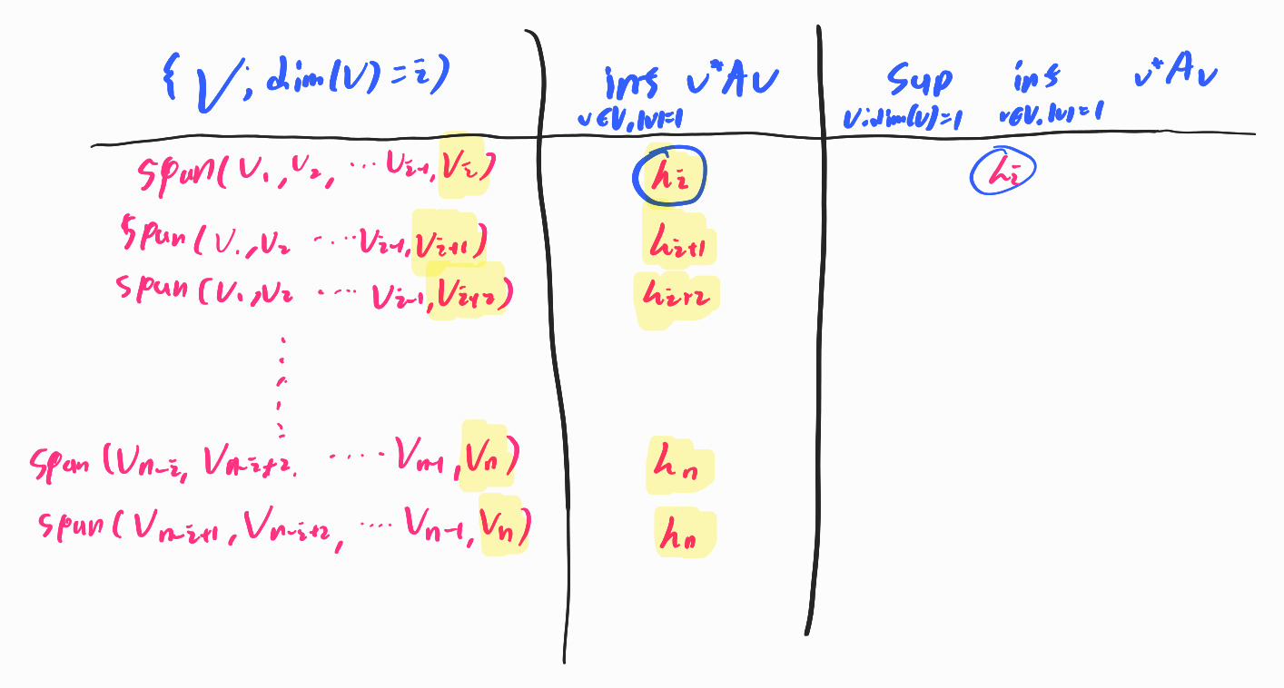
\[\lambda_i(A) = \underset{\dim (V) = i}{\sup} \underset{v \in V, \mid v \mid =1}{\inf} v^{\ast}Av\] \[\lambda_i(A) = \underset{\dim (V) = n-i+1}{\inf} \underset{v \in V, \mid v \mid =1}{\sup} v^{\ast}Av\]where V ranges over all subspaces of \(C^{n}\) with the indicated dimension
pf)
In first view, it is hard to understand what the theorem wants to talk about. Let me depict it. If we set \(A\) of first equation \(-A\), then we can naturally derive the second equation.(notice that \(\lambda_i(-A) = -\lambda_{n-i+1}(A)\)) So, let’s see the first one only.
We can assume the eigenvalues are critical points. We have \(Av_k =\lambda v_k \rightarrow v_k^{\ast}Av_k = \lambda_k v_k^{\ast}v_k=\lambda_k\).
Assume \(V = span(v_1,v_2,...,v_j)\), we can represent any vector \(v \in V\) as \(v = \sum_{k=1}^j \alpha_k v_k\).
And because of constraint \(\mid v \mid^2 = \mid \sum_{k=1}^{j} a_k v_k\mid^2 = \sum_{k=1}^{j} \mid \alpha_{k}\mid ^2 =1\). By using it, we can expand it as follow.
\[v^{\ast}Av = (\sum_k \alpha_k^{\ast} v_k^{\ast} )A(\sum_l \alpha_l v_j) = \sum_k \sum_l \alpha_k^{\ast}\alpha_l (v_{k}^{\ast} Av_l) = \sum_k \sum_l \alpha_k^{\ast} \alpha_l\lambda_l (v^{\ast}_k v_l) = \sum_k \lambda_k \mid \alpha_k \mid^2\]Because \(\sum \mid \alpha_k \mid ^2 =1\), we can consider \(v^{\ast}A v\) as value mixed by \(\lambda_k\) with portion of \(\mid \alpha_k \mid ^2\). Because \(\lambda_1 \geq \lambda_2 \geq ... \geq \lambda_j\), the infimum of \(\sum_{k=1}^j \lambda_k \mid \alpha_k \mid^2\) is \(\lambda_j\) when \(\alpha_k =\begin{cases} 1 \mbox{ if } k=j \\ 0 \mbox{ if } k\neq j \end{cases}\) .
In summary,\(\underset{v \in V, \mid v \mid =1}{\inf} v^{\ast}Av = \min(\{\lambda_j: \lambda_j \mbox{ is eigenvalue correspond with basis of } V \})\) where \(\lambda_j\) is the smallest eigenvalue correspond with the basis of \(V\). We can interpret the supremum as follow.
For a subspace \(V\) of \(V' =span(v_1,v_2,...,v_n)\), \(V\) could be represented as \(span(v_{n_1},v_{n_2},...,v_{n_i})\). For a fixed i, \(\underset{\dim (V) = i}{\sup} \underset{v \in V, \mid v \mid =1}{\inf} v^{\ast}Av\) becomes largest possible values among smallest eigenvalue of i number of combination of \(\lambda_1,\lambda_2,...,\lambda_n\). Therefore, it is naturally $\lambda_i$. Below figure depicts the logics to pick the supremum
If we substitute \(i=1\), then we can derive more intuitive result \(\lambda_1(A) = \underset{v \in V , \mid v \mid =1}{\sup} v^{\ast}Av\) and \(\lambda_n (A) = \underset{v \in V ,\mid v \mid =1}{\inf} v^{\ast}A v\). Therefore, we can derive following range.
Quadratic Form Theorem
For a Hermitian matrix \(A\) and unit vector \(v\), the inequaility \(\lambda_n\leq v^{\ast}Av \leq \lambda_1\) holds equivalently, \(v^{\ast}A v \in (\lambda_n , \lambda_1)\).
It means that the quadratic form of the matrix is bounded with its eigenvalues. By using the inequality, we can derive more interesting concepts.
Let \(v \in V\) be any vector and \(v' = \frac{v}{\parallel v \parallel_2}\), then we can get following result
\[\parallel Av \parallel_2 = (v^{\ast}A^\ast A v)^{1/2} = (v^{\ast} A^2 v)^{1/2} =\parallel v \parallel_2 (v'^{\ast} A^2 v')^{1/2} \leq \max (\mid \lambda_1\mid ,\mid \lambda_n \mid) \parallel v \parallel_2\]We can interpret it as the operator expand the magnitude of input values at most \(\lambda_1\) times.
Moreover, the definition of operator norm is \(\parallel A \parallel_{op} = \inf \{c : \parallel Av\parallel \leq c \parallel v \parallel\}\). Therefore, we could know that for complex vector Hilbert space with standard inner product \(\langle x , y\rangle = \sum x_i \overline{y_i}\), the operator norm \(\parallel A\parallel_{op}\) is \(\max (\mid \lambda_1\mid ,\mid \lambda_n \mid)\). Particularly, if
By using the spectral theorem, we can factorize the Hermitian matrix as \(A = \Gamma \Lambda \Gamma^{\ast}\) where \(\Gamma^{\ast}\Gamma =I\). It generate the equation \(tr(A) = tr(\Gamma \Lambda \Gamma^{\ast}) = tr(\Gamma^{\ast}\Gamma \Lambda) = tr(\Lambda)=\sum_{i=1}^n \lambda_i (A)\).
Then we can generate another equation that \(tr(A+B) = tr(A)+tr(B) \Rightarrow \sum_{i=1}^n \lambda_i(A+B)= \sum_{i=1}^n [\lambda_i(A)+\lambda_i(B)]\)
By using the fact that \(\lambda_1 (A) = \underset{\mid v \mid =1}{\sup} v^{\ast}Av\), we can get \(\lambda_1(A+B)\leq \lambda_1(A)+\lambda_1(B)\). Likewise, by fixing the dimension with \(i\), we can generalized the result as \(\lambda_{i}(A+B) \leq \lambda_i(A) + \lambda_i(B)\).
Like above, there is more complicated inequality. We can summarize them as follow.
- \(\lambda_{i}(A+B) \leq \lambda_i(A) + \lambda_i(B)\).
- Weyl Inequality : \(\lambda_1(A+B)+...+\lambda_k(A+B) \leq \lambda_1(A)+...+\lambda_k(A)+\lambda_1(B)+...+\lambda_k(B)\)
- Ky Fan Inequality : \(\lambda_{i+j-1}(A+B) \leq \lambda_i(A)+\lambda_{j}(B)\)
- Schur-Horn Inequality : \(\lambda_{n-k+1}(A) + ...+\lambda_n(A) \leq a_{i_1 i_1}+...+a_{i_k i_k} \leq \lambda_1(A)+...+\lambda_k(A)\) where \(i_k\) is increasing subsequence of \(\{1,2,...,n\}\)
If we use the first inequality, we can get \(\ \lambda_i (A+B) -\lambda_i(A) \mid \leq \parallel B \parallel _{op} = \parallel (A+B) -(A) \parallel_{op}\). This means that the functional \(\lambda_i (A)\) is Lipschitz continuous.
2.1 The Norms of Matrix
With the Eigenvalue, we can derive various norms of matrix.
The most important norm in the Euclidean Space and function space is Lp-norm class. Likewise, there is a class of norm which has a similar position in the Euclidean space and function space: p-Schatten norm (Sp-norm).
p-norm class
Lp norm of n-dimensional complex vector space (Space of scalar valued vectors)
For \(x =(x_1,x_2,x_3,...,x_n) , x_i \in \mathbb{C}\): n-dimensional complex vector space, the L-p norm \(\parallel x \parallel_p\) is defined as \(\parallel x \parallel_p = (\sum_{i=1}^n \mid x_i \mid ^p)^{1/p}\)
Lp norm of infinite dimensional complex vector space (Space of sequences)
For \(x =(x_1,x_2,x_3,...) , x_i \in \mathbb{C}\): infinite dimensional complex vector space, the L-p norm \(\parallel x \parallel_p\) is defined as \(\parallel x \parallel_p = (\sum_{i=1}^{\infty} \mid x_i \mid ^p)^{1/p}\)
Lp norm of functional space
For \(f \in H(N)\): functional space whose domain is space \(N\), the L-p norm \(\parallel f \parallel_p\) is defined as \(\parallel f \parallel_p = (\int_{N} \mid f(x)\mid ^p dx)^{1/p}\)
Sp norm of matrix space
For \(A = \{a_{ij}\}_{i,j=1}^{n}\): \(n \times n\) Hermitian Matrix, the S-p norm \(\parallel A \parallel_p = ( \sum_{i=1}^n \mid \lambda_i(A)\mid ^p)^{1/p} = \parallel \lambda \parallel_p\)
There is a special class of Sp norm. And this special cases are densely connected with the L-p norm.
p=1
For p=1, we can expand the norm as \(\parallel A \parallel_1 = \sum_{i=1}^n \mid \lambda_i(A) \mid=tr(\mid A \mid) =tr( (A A^{\ast})^{1/2}\). Therefore, S1 norm is actually trace of the matrix A. Therefore, it is also called as trace norm and denoted by \(\parallel A\parallel_{tr} = \parallel A \parallel_{1}\).
p=2
For p=2, we can expand the concepts as \(\parallel A \parallel_2 = (\sum_{i=1}^n \mid \lambda_{i}(A) \mid ^2 )^{1/2} = tr^{1/2}( \mid \Lambda \mid ^2) = tr^{1/2}(\mid A \mid ^2) = tr^{1/2}(A A^{\ast}) = \sum_{i=1}^n\sum_{j=1}^n \mid a_{ij}\mid ^2\)
As we can see, the S2 norm is actually the L2 norm regarding every element as vector. It is also called as Frobenius norm or Hilbert-Schmidt norm.
We can say that the S2 norm is most important norm of matrix by two reason.
The first reason is that we can calculate the derivatives of it very easily. For example, we can find \(\frac{d}{d A}\parallel A \parallel_2 = \{\frac{d}{d a_{ij}} \parallel A \parallel_2\}_{i,j} = 2\{a_{ij} \}_{ij} =2A\)
The second reason is that the S2 norm could be endowed with the inner product by defining \(\langle A ,B \rangle = tr(AB^{\ast})\). Therefore, the so-called S2 space \(\{A : \parallel A \parallel_2 < \infty\}\) is Hilbert Space. The inner product is called as Hilbert–Schmidt inner product.
p=\(\infty\)
For \(p = \infty\), the norm is defined as \(\parallel A \parallel_\infty = \parallel \lambda \parallel_{\infty} = \sup \mid \lambda \mid = \max(\mid \lambda_1\mid ,\mid \lambda_n \mid)\).
Therefore, it is operator norm mentioned above. The operator norm is one of the most important norm because it handles the essential property of operator in that the operator norm is the maximal expanding value.
There is a concepts of dual norm which states that the dual norm of \(\parallel f \parallel_p\) is \(\parallel f \parallel_q\) where \(\frac{1}{p}+\frac{1}{q}=1\). It could be used at various fields including optimization. The dual norm of the operator norm is the trace norm and vice versa. We can conjecture the connection between them by applying \(\frac{1}{1}+\frac{1}{\infty} \approx 1\).
2.2 Eigenvalue Deformation
The theory of random matrix usually make the random matrix \(A(t)\) as perturbed version \(A(t)=A+tB\). Therefore, to handle the random matrix easily, we have to build the derivatives of it.
If the eigenvalues are not repeated which is usual case, we say the Hermitian matrix has simplex spectrum.
It the Hermitian Matrix A is simplex, then the eigenvalue function \(\lambda_i(A)\) is smooth function i.e. infinitely differentiable. Let’s see the logics.
- If a Hermitian Matrix A is simple, then \(q_i\) in the characteristic function \(\prod_{i=1}^p (A - \lambda_i I)^{q_i} \approx prod_{i=1}^p (\lambda - \lambda_i I)^{q_i}\) is always one. Therefore, by simple calculation, we can know that \(\frac{\delta}{\delta \lambda} \prod_{i=1}^p (\lambda - \lambda_iI) \mid_{\lambda = \lambda_i} \neq 0\).
- By inverse function theorem which states that a function is locally differentiable and it derivatives is zero if and only if there exists a local inverse function and the derivative of the local inverse function is not zero, \(\frac{\delta A}{\delta \lambda_i}\neq 0 \rightarrow \frac{\delta \lambda_i}{\delta A}\neq 0\)
- Therefore, \(\lambda_i(A)\) is infinitely differentiable. Similarly, the eigenvector function \(\frac{\delta u_i(A)}{\delta A}\) is also smooth.
Therefore, we can derive derivatives of eigenvalue as follow.
\(A u_i = \lambda_i u_i\) and \(u_i^{\ast}u_i=1\)
Taking derivatives both of them, then we can get following equation.
\(\overset{\cdot}{A} u_i + A \overset{\cdot}{u}_i = \overset{\cdot}{\lambda_{i}} u_i + \lambda_i \overset{\cdot}{u_i}\) and \(\overset{\cdot}u_i^{\ast}u_i+u_i^{\ast}\overset{\cdot}u_i=0\)
The second relation gives us \(u_i^{\ast}\overset{\cdot}u_i=0\). By multiplying \(u_i^{\ast}\) on both sides of first equation, we can get Hadamard First Variation Formula.
\[u_i^{\ast}\overset{\cdot}{A}u_i+u_i^{\ast}A\overset{\cdot}{u_i} =\overset{\cdot}{\lambda_i}u_i^{\ast}u_i+\lambda_iu_i^{\ast}\overset{\cdot}{u_i}\] \[\Rightarrow u_i^{\ast}\overset{\cdot}{A}u_i +\lambda_i^{\ast}u_i^{\ast}\overset{\cdot}u_i=\overset{\cdot}{\lambda}_i+\lambda_i u_i^{\ast}\overset{\cdot}u_i\] \[\Rightarrow u_i^{\ast}\overset{\cdot}{A}u_i=\overset{\cdot}{\lambda}_i\]By using it, we can derive the derivatives of eigenvalue function \(\frac{d}{dt}\lambda_i(A+tB)=u_i(A+tB)^{\ast}Bu_i(A+tB)\)
Because it is also in \(u_i^{\ast}Bu_u \leq \parallel B\parallel_{OP}\), we can see that it is Lipschitz continuous.